DATA SCIENCE QUIZ 3 FINAL FLASHCARD SET

What is a JSON

an open standard format for creating and storing files or exchanging data that uses comprehensible and human-readable text made up of attributes and serializable values

3 Pros of JSONs / Why are JSONs used

1. It is easy for humans to read and write.

2. It is easy for machines to parse and generate.

3. It is commonly used for APIs (Application Program Interface) to share data.

write the format of a JSON containing 4 variables (name, age, city, hobbies) for a 30 year old man named John for New York who likes to read, hike, and code,

what is a Key-Value Pair in a JSON?

Each pair consists of a key (string) and a value (can be string, number, boolean, array, or another object).

Example: key = “name”: , value = “John”

Curly Braces {} in a JSON

Enclose an object, which is a collection of key-value pairs (one row)

Square Brackets [] in a JSON

These enclose an array, which is an ordered list of values (all rows)

How do JSON files relate to data frames

Originally, a JSON is treated as a string of characters

Use fromJSON(simplifyVector = TRUE)

If it is an array that satisfies the constraints of a data frame, it may be able to simplify to data frame and each element of the array is one row of a dataset, each key is a column

Otherwise it is treated as a named list with elements many not all of the same length (not a data frame)

fromJSON(json, simplifyVector = FALSE) versus fromJSON(json, simplifyVector = TRUE)

simplifyVector = FALSE:

• always possible

• provides a list

[[1]]
[[1]]$Name
[1] "Mario"

[[1]]$Age
[1] 32

[[1]]$Occupation
[1] "Plumber"


[[2]]
[[2]]$Name
[1] "Peach"

[[2]]$Age
[1] 21

[[2]]$Occupation
[1] "Princess"

simplifyVector = TRUE:

• Only possible If it is an array that satisfies the constraints of a data frame,

• Simplify to data frame

Name Age Occupation
1  Mario  32    Plumber
2  Peach  21   Princess
3   <NA>  NA       <NA>
4 Bowser  NA      Koopa

How many main parent elements are in this JSON?

{
    "result_count": 3, 
    "results": [
        {
            "_href": "/ws.v1/lswitch/3ca2d5ef-6a0f-4392-9ec1-a6645234bc55", 
            "_schema": "/ws.v1/schema/LogicalSwitchConfig", 
            "type": "LogicalSwitchConfig"
        }, 
        {
            "_href": "/ws.v1/lswitch/81f51868-2142-48a8-93ff-ef612249e025", 
            "_schema": "/ws.v1/schema/LogicalSwitchConfig", 
            "type": "LogicalSwitchConfig"
        }, 
        {
            "_href": "/ws.v1/lswitch/9fed3467-dd74-421b-ab30-7bc9bfae6248", 
            "_schema": "/ws.v1/schema/LogicalSwitchConfig", 
            "type": "LogicalSwitchConfig"
        }
    ]

2: results_count and results

If you converted this to R data types, what structure makes the most sense to use?

{
    "result_count": 3, 
    "results": [
        {
            "_href": "/ws.v1/lswitch/3ca2d5ef-6a0f-4392-9ec1-a6645234bc55", 
            "_schema": "/ws.v1/schema/LogicalSwitchConfig", 
            "type": "LogicalSwitchConfig"
        }, 
        {
            "_href": "/ws.v1/lswitch/81f51868-2142-48a8-93ff-ef612249e025", 
            "_schema": "/ws.v1/schema/LogicalSwitchConfig", 
            "type": "LogicalSwitchConfig"
        }, 
        {
            "_href": "/ws.v1/lswitch/9fed3467-dd74-421b-ab30-7bc9bfae6248", 
            "_schema": "/ws.v1/schema/LogicalSwitchConfig", 
            "type": "LogicalSwitchConfig"
        }
    ]

Named list of 2 elements ($result_count -  numeric class, $results - data frame class)

Focus only on the results. What does each { XXX } represent?

{
    "result_count": 3, 
    "results": [
        {
            "_href": "/ws.v1/lswitch/3ca2d5ef-6a0f-4392-9ec1-a6645234bc55", 
            "_schema": "/ws.v1/schema/LogicalSwitchConfig", 
            "type": "LogicalSwitchConfig"
        }, 
        {
            "_href": "/ws.v1/lswitch/81f51868-2142-48a8-93ff-ef612249e025", 
            "_schema": "/ws.v1/schema/LogicalSwitchConfig", 
            "type": "LogicalSwitchConfig"
        }, 
        {
            "_href": "/ws.v1/lswitch/9fed3467-dd74-421b-ab30-7bc9bfae6248", 
            "_schema": "/ws.v1/schema/LogicalSwitchConfig", 
            "type": "LogicalSwitchConfig"
        }
    ]

One row of data

What is an API?

Application Programming Interface describes a general class of tool that allows computer software, rather than humans, to interact with an organization’s data.

• Application refers to software.

• Interface: a contract of service between two applications

  • This contract defines how the two communicate with each other using requests and responses

  • Does not see it in a graphical format like humans

Is there a standard way to access APIs?

Every API has documentation for how software developers should structure requests for data / information and in what format to expect responses.

• This makes it more ethical

• There is not one standard way to access an API

Web APIs

Web Application Programming Interfaces, which focus on transmitting requests and responses for raw data through a web browser.

• Our browsers communicate with web servers using a technology called HTTP or Hypertext Transfer Protocol.

• Programming languages such as R can also use HTTP to communicate with web servers.

https://api.census.gov
what is the base url, the scheme and the hostname

• https://api.census.gov is the base URL.

• http:// is the scheme (tells your browser or program how to communicate with the web server)

• api.census.gov is the hostname or host address, which is a name that identifies the web server that will process the request.

https://api.census.gov/data/2019/acs/acs1?get=NAME,B02015_009E,B02015_009M&for=state:*

What is the file path?

Tells the web server how to get to the desired resource.

• data/2019/acs/acs1

What is the query string?

https://api.census.gov/data/2019/acs/acs1?get=NAME,B02015_009E,B02015_009M&for=state:*

it provides the parameters for the function you would like to call

?get=NAME,B02015_009E, B02015_009M&for=state:*

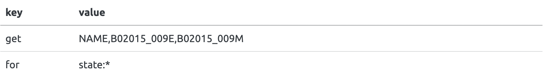
How are string / key pairs formatted in a query string?

This is a string of key-value pairs separated by &.

That is, the general structure of this part is key1=value1&key2=value2.

In R, it is easiest to access Web APIs through…?

A wrapper package, an R package written specifically for a particular Web API

Many APIs require users to obtain a ____ to use their services. Why?

key

This lets organizations keep track of what data is being used

it also rate limits their API and ensures programs don’t make too many requests per day/minute/hour.

API key rate limits

Ensures programs don’t make too many requests per day/minute/hour

Percent encoding in a url

URL encoding replaces unsafe ASCII characters with a "%" followed by two hexadecimal digits. URLs cannot contain spaces. URL encoding normally replaces a space with a plus (+) sign or with %20.

httr2::request()

creates an API request object using the base URL

httr2::req_url_path_append()

builds up the URL by adding path components separated by /

httr2::req_url_query()
(4 arguments)

adds the ? separating the endpoint from the query and sets the key-value pairs in the query

get = c("variable1", "variable2")

`for` = I(“row: rowname”) or I(“row: *”)

• I() funtion inhibits parsing of special characters like : and *

• don't forget backticks

key = api key name

.multi = “comma” controls how multiple values for a given key are combined.

use httr2 to build the URL https://api.census.gov/data/2019/acs/acs1?get=NAME,B02015_009E,B02015_009M&for=state:*

req <- request("https://api.census.gov") %>% 
    req_url_path_append("data") %>% 
    req_url_path_append("2019") %>% 
    req_url_path_append("acs") %>% 
    req_url_path_append("acs1") %>% 
    req_url_query(get = c("NAME", "B02015_009E", "B02015_009M"), `for` = I("state:*"), key = census_api_key, .multi = "comma")

why would we use httr2 instead of just writing the URL string?

• To generalize this code with functions!

• To handle special characters

  • e.g., query parameters might have spaces, which need to be represented in a particular way in a URL (URLs can’t contain spaces)

Once we’ve fully constructed our request, we can use _____ to send out the API request and get a response.

req_perform()

What format is the API response in? What can use do?

JSON

resp_body_json(simplifyVector = TRUE) creates a dataframe

• Without simplifyVector = TRUE, the JSON is read in as a list.

API Documentation - what to look for

NOT SURE WHAT TO PUT HERE

Consider the following url (uniform resource locator):

 

https://www.tutorialspoint.com/html/understanding_url_tutorial.htm

 

Which part is the "Scheme"?

https://

Consider the following url (uniform resource locator):

 

https://www.tutorialspoint.com/html/understanding_url_tutorial.htm

 

Which part is the "Host Address"?

www.tutorialspoint.com

Consider the following url (uniform resource locator):

 

https://www.tutorialspoint.com/html/understanding_url_tutorial.htm

 

Which part is the "File Path"?

/html/understanding_url_tutorial.htm

Consider the following url (uniform resource locator):

 

https://www.tutorialspoint.com/html/html_text_links.htm#top

 

Which part is the "fragment identifier"?

#top

Consider the following url (uniform resource locator):

 

https://www.tutorialspoint.com/cgi-bin/search.cgi?searchTerm=HTML

 

Which part is the "query"?

searchTerm=HTML

url_encode() in urltools is useful for…

converting a string to a percentage-encoded URL

url_decode() in urltools is useful for…

taking percentage-encoded URLS and converting it to a string

When to use web scraping

Whenever an API is available for your project, you should default to getting data from the API. Sometimes an API will not be available, and web scraping is another means of getting data.

what is web scraping

Web scraping describes the use of code to extract information displayed on a web page.

Ethics of web scraping 

robots.txt is a file that some websites will publish to clarify what can and cannot be scraped and other constraints about scraping. When a website publishes this file, this we need to comply with the information in it for moral and legal reasons.

robots.txt: user-agent

It determines who's allowed to do web scraping.

If User-agent has a wildcard (*), that means everyone is allowed to crawl. If containing a specific name, such as AdsBot-Google, that represents only Google is allowed in this case.

robots: Allow / Disallow

When Disallow has no value, all pages are allowed for scraping. If you see /, that implies every single page is disallowed. In case you'd see a path or file name, such as /folder/ or /file.html, we're being pointed out what shouldn't be crawled.

An alternative instruction for Disallow is Allow, which states the only resources you should visit.

Crawl Delay

Crawl-delay sets the speed in seconds at which you can scrape each new resource. This helps websites prevent server overload, whose consequence would be slowing down the site for human visitors

HTML structure

HTML (hypertext markup language) is the formatting language used to create webpages. HTML has a hierarchical structure formed by elements which consist of a start tag (e.g. <tag>), optional attributes (id='first'), an end tag1 (like </tag>), and contents (everything in between the start and end tag).

HTML: Elements

consist of a start tag (e.g. <tag>) and end with an end tag (e.g. </tag>)

there are over 100 HTML elements. Some of the most important are:

Every HTML page must be in an <html> element, and it must have two children: <head>, which contains document metadata like the page title, and <body>, which contains the content you see in the browser.

HTML: tags

Tags (common tag: <p> <img> <a> <h1> <h2> <div>

Block tags like <h1> (heading 1), <p> (paragraph), and <ol> (ordered list) form the overall structure of the page.

Inline tags like <b> (bold), <i> (italics), and <a> (links) formats text inside block tags.

HTML: Attributes

Tags can have named attributes which look like name1='value1' name2='value2'. Two of the most important attributes are id and class, which are used in conjunction with CSS (Cascading Style Sheets) to control the visual appearance of the page. These are often useful when scraping data off a page.

HTML: Contents of an element

Most elements can have content in between their start and end tags. This content can either be text or more elements. For example, the following HTML contains paragraph of text, with one word in bold.

Hi! My name is Hadley.

The children of a node refers only to elements, so the <p> element above has one child, the <b> element. The <b> element has no children, but it does have contents (the text “name”).

Some elements, like <img> can’t have children. These elements depend solely on attributes for their behavior.

read_html()

Reads and parses the HTML content of a webpage. First step to load the page into R.

html_elements()

enables you to select and extract specific HTML elements from a webpage based on their tags, classes, or attributes.

Selects nodes (elements) from the HTML using a CSS selector.

To extract specific sections, tags, or components of the page.

html_text()

Extracts text content from selected HTML elements, stripping out any HTML tags.

html_attr()

Extracts specific attributes from HTML elements, such as href or class. This is useful for obtaining metadata or links from the elements.

CSS manually: tags

target all elements of a specific type. ex: p

CSS manually: #id

A single element with a specific ID. syntax ex: #header

CSS manually: .class

All elements with a specific class. syntax ex: .highlight

CSS Selector Gadget

Selector Gadget is a Chrome extension that helps you find CSS selectors visually. Copy the suggested CSS selector and use it in your code or for scraping.

Cloud DBMS

like Snowflake, Amazon’s RedShift, and Google’s BigQuery, are similar to client server DBMS’s, but they run in the cloud. This means that they can easily handle extremely large datasets and can automatically provide more compute resources as needed.

Client-Server DBMS

run on a powerful central server, which you connect to from your computer (the client). They are great for sharing data with multiple people in an organization. Popular client-server DBMS’s include PostgreSQL, MariaDB, SQL Server, and Oracle.

In-Process DBMS

like SQLite or duckdb, run entirely on your computer. They’re great for working with large datasets where you’re the primary user.

DBs row & column orientation

Most classical databases are optimized for rapidly collecting data, not analyzing existing data. These databases are called row-oriented because the data is stored row-by-row, rather than column-by-column like R. More recently, there’s been much development of column-oriented databases that make analyzing the existing data much faster.

2 differences between df and db:

• Database tables are stored on disk and can be arbitrarily large. Data frames are stored in memory, and are fundamentally limited (although that limit is still plenty large for many problems).

• Database tables almost always have indexes. Much like the index of a book, a database index makes it possible to quickly find rows of interest without having to look at every single row. Data frames and tibbles don’t have indexes, but data.tables do, which is one of the reasons that they’re so fast.

What is a DBI?

DataBase Interface that provides a set of generic functions that connect to the database, upload data, run SQL queries, etc.

How do you create a DB connection

you create a database connection using DBI::dbConnect()examples: con <- DBI::dbConnect( RMariaDB::MariaDB(), username = "foo" )

con <- DBI::dbConnect( RPostgres::Postgres(), hostname = "databases.mycompany.com", port = 1234 ), and if using duckb con <- DBI::dbConnect(duckdb::duckdb(), dbdir = "duckdb")

What is the next step after establishing a connection?

Using dbWriteTable() to create a db! The simplest usage of dbWriteTable() needs three arguments: a database connection, the name of the table to create in the database, and a data frame of data.

dbWriteTable(con, "mpg", ggplot2::mpg)
dbWriteTable(con, "diamonds", ggplot2::diamonds)

Other initial dbi functions

You can check that the data is loaded correctly by using a couple of other DBI functions: dbListTables() lists all tables in the database³ and dbReadTable() retrieves the contents of a table. dbReadTable() returns a data.frame so we use as_tibble() to convert it into a tibble so that it prints nicely.

dplyr within databases

dbplyr is a dplyr backend, which means that you keep writing dplyr code but the backend executes it differently. In this, dbplyr translates to SQL; other backends include dtplyr which translates to data.table, and multidplyr which executes your code on multiple cores.

database interactions/selecting data

There are two other common ways to interact with a database. First, many corporate databases are very large so you need some hierarchy to keep all the tables organized. In that case you might need to supply a schema, or a catalog and a schema, in order to pick the table you’re interested in:

diamonds_db <- tbl(con, in_schema("sales", "diamonds"))
diamonds_db <- tbl(con, in_catalog("north_america", "sales", "diamonds"))

Other times you might want to use your own SQL query as a starting point:

diamonds_db <- tbl(con, sql("SELECT * FROM diamonds"))

SQL within R

You can see the SQL code generated by the dplyr function show_query(). To get all the data back into R, you call collect(). Behind the scenes, this generates the SQL, calls dbGetQuery() to get the data, then turns the result into a tibble:

big_diamonds <- big_diamonds_db |> 
  collect()
big_diamonds
#> # A tibble: 1,655 × 5
#>   carat cut       color clarity price
#>   <dbl> <fct>     <fct> <fct>   <int>
#> 1  1.54 Premium   E     VS2     15002
#> 2  1.19 Ideal     F     VVS1    15005
#> 3  2.1  Premium   I     SI1     15007
#> 4  1.69 Ideal     D     SI1     15011
#> 5  1.5  Very Good G     VVS2    15013
#> 6  1.73 Very Good G     VS1     15014
#> # ℹ 1,649 more rows

SQL components

The top-level components of SQL are called statements. Common statements include CREATE for defining new tables, INSERT for adding data, and SELECT for retrieving data. We will focus on SELECT statements, also called queries, because they are almost exclusively what you’ll use as a data scientist.

A query is made up of clauses. There are five important clauses: SELECT, FROM, WHERE, ORDER BY, and GROUP BY. Every query must have the SELECT⁴ and FROM⁵ clauses and the simplest query is SELECT * FROM table, which selects all columns from the specified table . This is what dbplyr generates for an unadulterated table

WHERE and ORDER BY

control which rows are included and how they are ordered:

flights |> 
  filter(dest == "IAH") |> 
  arrange(dep_delay) |>
  show_query()
#> <SQL>
#> SELECT flights.*
#> FROM flights
#> WHERE (dest = 'IAH')
#> ORDER BY dep_delay

GROUP BY

converts the query to a summary, causing aggregation to happen:

flights |> 
  group_by(dest) |> 
  summarize(dep_delay = mean(dep_delay, na.rm = TRUE)) |> 
  show_query()
#> <SQL>
#> SELECT dest, AVG(dep_delay) AS dep_delay
#> FROM flights
#> GROUP BY dest

differences between dplyr verbs and SELECT clauses

• In SQL, case doesn’t matter: you can write select, SELECT, or even SeLeCt. In this book we’ll stick with the common convention of writing SQL keywords in uppercase to distinguish them from table or variables names.

• In SQL, order matters: you must always write the clauses in the order SELECT, FROM, WHERE, GROUP BY, ORDER BY. Confusingly, this order doesn’t match how the clauses are actually evaluated which is first FROM, then WHERE, GROUP BY, SELECT, and ORDER BY.

SELECT

The SELECT clause is the workhorse of queries and performs the same job as select(), mutate(), rename(), relocate(), and, as you’ll learn in the next section, summarize().

select(), rename(), and relocate() have very direct translations to SELECT as they just affect where a column appears (if at all) along with its name:

planes |> 
  select(tailnum, type, manufacturer, model, year) |> 
  show_query()
#> <SQL>
#> SELECT tailnum, "type", manufacturer, model, "year"
#> FROM planes

planes |> 
  select(tailnum, type, manufacturer, model, year) |> 
  rename(year_built = year) |> 
  show_query()
#> <SQL>
#> SELECT tailnum, "type", manufacturer, model, "year" AS year_built
#> FROM planes

planes |> 
  select(tailnum, type, manufacturer, model, year) |> 
  relocate(manufacturer, model, .before = type) |> 
  show_query()
#> <SQL>
#> SELECT tailnum, manufacturer, model, "type", "year"
#> FROM planes

SQL renaming

In SQL terminology renaming is called aliasing and is done with AS. Note that unlike mutate(), the old name is on the left and the new name is on the right.

reserved words in SQL

In the examples above note that "year" and "type" are wrapped in double quotes. That’s because these are reserved words in duckdb, so dbplyr quotes them to avoid any potential confusion between column/table names and SQL operators.

When working with other databases you’re likely to see every variable name quoted because only a handful of client packages, like duckdb, know what all the reserved words are, so they quote everything to be safe.

SELECT "tailnum", "type", "manufacturer", "model", "year"
FROM "planes"

Some other database systems use backticks instead of quotes:

SELECT `tailnum`, `type`, `manufacturer`, `model`, `year`
FROM `planes`

mutate in SQL

The translations for mutate() are similarly straightforward: each variable becomes a new expression in SELECT:

flights |> 
  mutate(
    speed = distance / (air_time / 60)
  ) |> 
  show_query()
#> <SQL>
#> SELECT flights.*, distance / (air_time / 60.0) AS speed
#> FROM flights

SQL WHERE

filter() is translated to the WHERE clause:
flights |> 
  filter(dest == "IAH" | dest == "HOU") |> 
  show_query()
#> <SQL>
#> SELECT flights.*
#> FROM flights
#> WHERE (dest = 'IAH' OR dest = 'HOU')

flights |> 
  filter(arr_delay > 0 & arr_delay < 20) |> 
  show_query()
#> <SQL>
#> SELECT flights.*
#> FROM flights
#> WHERE (arr_delay > 0.0 AND arr_delay < 20.0)

There are a few important details to note here:

• | becomes OR and & becomes AND.

• SQL uses = for comparison, not ==. SQL doesn’t have assignment, so there’s no potential for confusion there.

• SQL uses only '' for strings, not "". In SQL, "" is used to identify variables, like R’s ``

SQL IN

Another useful SQL operator is IN, which is very close to R’s %in%:

flights |> 
  filter(dest %in% c("IAH", "HOU")) |> 
  show_query()
#> <SQL>
#> SELECT flights.*
#> FROM flights
#> WHERE (dest IN ('IAH', 'HOU'))

SQL NULL VS NA

SQL uses NULL instead of NA. NULLs behave similarly to NAs. The main difference is that while they’re “infectious” in comparisons and arithmetic, they are silently dropped when summarizing. dbplyr will remind you about this behavior the first time you hit it:

flights |> 
  group_by(dest) |> 
  summarize(delay = mean(arr_delay))
#> Warning: Missing values are always removed in SQL aggregation functions.
#> Use `na.rm = TRUE` to silence this warning
#> This warning is displayed once every 8 hours.
#> # Source:   SQL [?? x 2]
#> # Database: DuckDB v1.2.1 [unknown@Linux 6.8.0-1021-azure:R 4.4.3/:memory:]
#>   dest  delay
#>   <chr> <dbl>
#> 1 ATL   11.3 
#> 2 CLT    7.36
#> 3 MCO    5.45
#> 4 MDW   12.4 
#> 5 HOU    7.18
#> 6 SDF   12.7 
#> # ℹ more rows

HAVING vs. WHERE in SQL

Note that if you filter() a variable that you created using a summarize, dbplyr will generate a HAVING clause, rather than a WHERE clause. This is a one of the idiosyncrasies of SQL: WHERE is evaluated before SELECT and GROUP BY, so SQL needs another clause that’s evaluated afterwards.

ORDER BY

Ordering rows involves a straightforward translation from arrange() to the ORDER BY clause:

flights |> 
  arrange(year, month, day, desc(dep_delay)) |> 
  show_query()
#> <SQL>
#> SELECT flights.*
#> FROM flights
#> ORDER BY "year", "month", "day", dep_delay DESC

Notice how desc() is translated to DESC: this is one of the many dplyr functions whose name was directly inspired by SQL.

Subquery

A subquery is just a query used as a data source in the FROM clause, instead of the usual table.

dbplyr typically uses subqueries to work around limitations of SQL. For example, expressions in the SELECT clause can’t refer to columns that were just created. That means that the following (silly) dplyr pipeline needs to happen in two steps: the first (inner) query computes year1 and then the second (outer) query can compute year2.

flights |> 
  mutate(
    year1 = year + 1,
    year2 = year1 + 1
  ) |> 
  show_query()
#> <SQL>
#> SELECT q01.*, year1 + 1.0 AS year2
#> FROM (
#>   SELECT flights.*, "year" + 1.0 AS year1
#>   FROM flights
#> ) q01

Order of SELECT and FROM in SQL

You’ll also see this if you attempted to filter() a variable that you just created. Remember, even though WHERE is written after SELECT, it’s evaluated before it

Joins

The main thing to notice here is the syntax: SQL joins use sub-clauses of the FROM clause to bring in additional tables, using ON to define how the tables are related.

dplyr’s names for these functions are so closely connected to SQL that you can easily guess the equivalent SQL for inner_join(), right_join(), and full_join():

SELECT flights.*, "type", manufacturer, model, engines, seats, speed
FROM flights
INNER JOIN planes ON (flights.tailnum = planes.tailnum)

SELECT flights.*, "type", manufacturer, model, engines, seats, speed
FROM flights
RIGHT JOIN planes ON (flights.tailnum = planes.tailnum)

SELECT flights.*, "type", manufacturer, model, engines, seats, speed
FROM flights
FULL JOIN planes ON (flights.tailnum = planes.tailnum)

Window Funcgitons

The translation of summary functions becomes more complicated when you use them inside a mutate() because they have to turn into so-called window functions. In SQL, you turn an ordinary aggregation function into a window function by adding OVER after it:

flights |> 
  group_by(year, month, day) |>  
  mutate_query(
    mean = mean(arr_delay, na.rm = TRUE),
  )
#> <SQL>
#> SELECT
#>   "year",
#>   "month",
#>   "day",
#>   AVG(arr_delay) OVER (PARTITION BY "year", "month", "day") AS mean
#> FROM flights

In SQL, the GROUP BY clause is used exclusively for summaries so here you can see that the grouping has moved from the PARTITION BY argument to OVER.

Window functions include all functions that look forward or backwards, like lead() and lag() which look at the “previous” or “next” value respectively:

flights |> 
  group_by(dest) |>  
  arrange(time_hour) |> 
  mutate_query(
    lead = lead(arr_delay),
    lag = lag(arr_delay)
  )
#> <SQL>
#> SELECT
#>   dest,
#>   LEAD(arr_delay, 1, NULL) OVER (PARTITION BY dest ORDER BY time_hour) AS lead,
#>   LAG(arr_delay, 1, NULL) OVER (PARTITION BY dest ORDER BY time_hour) AS lag
#> FROM flights
#> ORDER BY time_hour

Intrinsic order of SQL output

Here it’s important to arrange() the data, because SQL tables have no intrinsic order. In fact, if you don’t use arrange() you might get the rows back in a different order every time! Notice for window functions, the ordering information is repeated: the ORDER BY clause of the main query doesn’t automatically apply to window functions.

if_else in SQL

flights |> 
  mutate_query(
    description = if_else(arr_delay > 0, "delayed", "on-time")
  )
#> <SQL>
#> SELECT CASE WHEN (arr_delay > 0.0) THEN 'delayed' WHEN NOT (arr_delay > 0.0) THEN 'on-time' END AS description
#> FROM flights
flights |> 
  mutate_query(
    description = 
      case_when(
        arr_delay < -5 ~ "early", 
        arr_delay < 5 ~ "on-time",
        arr_delay >= 5 ~ "late"
      )
  )
#> <SQL>
#> SELECT CASE
#> WHEN (arr_delay < -5.0) THEN 'early'
#> WHEN (arr_delay < 5.0) THEN 'on-time'
#> WHEN (arr_delay >= 5.0) THEN 'late'
#> END AS description
#> FROM flights

CASE WHEN is also used for some other functions that don’t have a direct translation from R to SQL. A good example of this is cut():

functional programming

often called functional programming tools because they are built around functions that take other functions as inputs. Learning functional programming can easily veer into the abstract, but in this chapter we’ll keep things concrete by focusing on three common tasks: modifying multiple columns, reading multiple files, and saving multiple objects.

inputs of across()

across() has three particularly important arguments, which we’ll discuss in detail in the following sections. You’ll use the first two every time you use across(): the first argument, .cols, specifies which columns you want to iterate over, and the second argument, .fns, specifies what to do with each column. You can use the .names argument when you need additional control over the names of output columns, which is particularly important when you use across() with mutate(). you can use functions like starts_with() and ends_with() to select columns based on their name.

There are two additional selection techniques that are particularly useful for across(): everything() and where(). everything() is straightforward: it selects every (non-grouping) column: df |> group_by(grp) |> summarize(across(everything(), median))

where()

where() allows you to select columns based on their type:

• where(is.numeric) selects all numeric columns.

• where(is.character) selects all string columns.

• where(is.Date) selects all date columns.

• where(is.POSIXct) selects all date-time columns.

• where(is.logical) selects all logical columns.

Just like other selectors, you can combine these with Boolean algebra. For example, !where(is.numeric) selects all non-numeric columns, and starts_with("a") & where(is.logical) selects all logical columns whose name starts with “a”

calling functions in across()

The second argument to across() defines how each column will be transformed. In simple cases, as above, this will be a single existing function. This is a pretty special feature of R: we’re passing one function (median, mean, str_flatten, …) to another function (across). This is one of the features that makes R a functional programming language.

It’s important to note that we’re passing this function to across(), so across() can call it; we’re not calling it ourselves. That means the function name should never be followed by (). If you forget, you’ll get an error:

df |> 
  group_by(grp) |> 
  summarize(across(everything(), median()))
#> Error in `summarize()`:
#> ℹ In argument: `across(everything(), median())`.
#> Caused by error in `median.default()`:
#> ! argument "x" is missing, with no default

This error arises because you’re calling the function with no input, e.g.:

median()
#> Error in median.default(): argument "x" is missing, with no default

calling a function inside of across()

It would be nice if we could pass along na.rm = TRUE to median() to remove these missing values. To do so, instead of calling median() directly, we need to create a new function that calls median() with the desired arguments:

df_miss |> 
  summarize(
    across(a:d, function(x) median(x, na.rm = TRUE)),
    n = n()
  )
#> # A tibble: 1 × 5
#>       a     b      c     d     n
#>   <dbl> <dbl>  <dbl> <dbl> <int>
#> 1 0.139 -1.11 -0.387  1.15     5

anonymous functions in across()

This is a little verbose, so R comes with a handy shortcut: for this sort of throw away, or anonymous¹, function you can replace function with \²:

df_miss |> 
  summarize(
    across(a:d, \(x) median(x, na.rm = TRUE)),
    n = n()
  )

multiple functions in across()

When we remove the missing values from the median(), it would be nice to know just how many values were removed. We can find that out by supplying two functions to across(): one to compute the median and the other to count the missing values. You supply multiple functions by using a named list to .fns:

df_miss |> 
  summarize(
    across(a:d, list(
      median = \(x) median(x, na.rm = TRUE),
      n_miss = \(x) sum(is.na(x))
    )),
    n = n()
  )

naming through across()

The result of across() is named according to the specification provided in the .names argument. We could specify our own if we wanted the name of the function to come first³:

df_miss |> 
  summarize(
    across(
      a:d,
      list(
        median = \(x) median(x, na.rm = TRUE),
        n_miss = \(x) sum(is.na(x))
      ),
      .names = "{.fn}_{.col}"
    ),
    n = n(),
  )
#> # A tibble: 1 × 9
#>   median_a n_miss_a median_b n_miss_b median_c n_miss_c median_d n_miss_d
#>      <dbl>    <int>    <dbl>    <int>    <dbl>    <int>    <dbl>    <int>
#> 1    0.139        1    -1.11        1   -0.387        2     1.15        0
#> # ℹ 1 more variable: n <int>

Coalesce()

Given a set of vectors, coalesce() finds the first non-missing value at each position. It's inspired by the SQL COALESCE function which does the same thing for SQL NULLs.

Usage

coalesce(..., .ptype = NULL, .size = NULL)

across() and filtering

across() is a great match for summarize() and mutate() but it’s more awkward to use with filter(), because you usually combine multiple conditions with either | or &. It’s clear that across() can help to create multiple logical columns, but then what? So dplyr provides two variants of across() called if_any() and if_all():

# same as df_miss |> filter(is.na(a) | is.na(b) | is.na(c) | is.na(d))
df_miss |> filter(if_any(a:d, is.na))
#> # A tibble: 4 × 4
#>        a      b      c     d
#>    <dbl>  <dbl>  <dbl> <dbl>
#> 1  0.434 -1.25  NA     1.60 
#> 2 NA     -1.43  -0.297 0.776
#> 3 -0.156 -0.980 NA     1.15 
#> 4  1.11  NA     -0.387 0.704

# same as df_miss |> filter(is.na(a) & is.na(b) & is.na(c) & is.na(d))
df_miss |> filter(if_all(a:d, is.na))
#> # A tibble: 0 × 4
#> # ℹ 4 variables: a <dbl>, b <dbl>, c <dbl>, d <dbl>

across() in functions

across() is particularly useful to program with because it allows you to operate on multiple columns. For example, Jacob Scott uses this little helper which wraps a bunch of lubridate functions to expand all date columns into year, month, and day columns:

expand_dates <- function(df) {
  df |> 
    mutate(
      across(where(is.Date), list(year = year, month = month, day = mday))
    )
}

df_date <- tibble(
  name = c("Amy", "Bob"),
  date = ymd(c("2009-08-03", "2010-01-16"))
)

df_date |> 
  expand_dates()
#> # A tibble: 2 × 5
#>   name  date       date_year date_month date_day
#>   <chr> <date>         <dbl>      <dbl>    <int>
#> 1 Amy   2009-08-03      2009          8        3
#> 2 Bob   2010-01-16      2010          1       16

Pivoting with across()

an interesting connection between across() and pivot_longer() (Section 5.3). In many cases, you perform the same calculations by first pivoting the data and then performing the operations by group rather than by column. For example, take this multi-function summary:

df |> 
  summarize(across(a:d, list(median = median, mean = mean)))
#> # A tibble: 1 × 8
#>   a_median a_mean b_median b_mean c_median c_mean d_median d_mean
#>      <dbl>  <dbl>    <dbl>  <dbl>    <dbl>  <dbl>    <dbl>  <dbl>
#> 1   0.0380  0.205  -0.0163 0.0910    0.260 0.0716    0.540  0.508

We could compute the same values by pivoting longer and then summarizing:

long <- df |> 
  pivot_longer(a:d) |> 
  group_by(name) |> 
  summarize(
    median = median(value),
    mean = mean(value)
  )
long
#> # A tibble: 4 × 3
#>   name   median   mean
#>   <chr>   <dbl>  <dbl>
#> 1 a      0.0380 0.205 
#> 2 b     -0.0163 0.0910
#> 3 c      0.260  0.0716
#> 4 d      0.540  0.508

And if you wanted the same structure as across() you could pivot again:

long |> 
  pivot_wider(
    names_from = name,
    values_from = c(median, mean),
    names_vary = "slowest",
    names_glue = "{name}_{.value}"
  )
#> # A tibble: 1 × 8
#>   a_median a_mean b_median b_mean c_median c_mean d_median d_mean
#>      <dbl>  <dbl>    <dbl>  <dbl>    <dbl>  <dbl>    <dbl>  <dbl>
#> 1   0.0380  0.205  -0.0163 0.0910    0.260 0.0716    0.540  0.508

reading in multiple files in 3 steps

There are three basic steps: use list.files() to list all the files in a directory, then use purrr::map() to read each of them into a list, then use purrr::list_rbind() to combine them into a single data frame. in a pipeline it would look like this: paths |> map(readxl::read_excel) |> list_rbind()