Landscape Evolution, Bedrock Rivers and Tectonic Geomorphology, Important Equations Review

- Identify knickpoints and assess their origin from various datasets and transformations (longitudinal profiles, slope/area space, geologic map and history) - Understand the drivers of landscape evolution on passive margin landscapes like the Appalachian Mountains - Evaluate the theories for the formation of wind and water gaps given what we know about fluvial geomorphology. - Define the essential components of a laboratory or numerical landscape, including initial and boundary conditions, focusing on the physical features and processes that need to be represented - Explain how topographic change can be mathematically/numerically represented through processes such as advection, diffusion, and uplift, focusing on the basic principles behind each process. - Debate the benefits and drawbacks of numerical and physical experiments in understanding landscape evolution

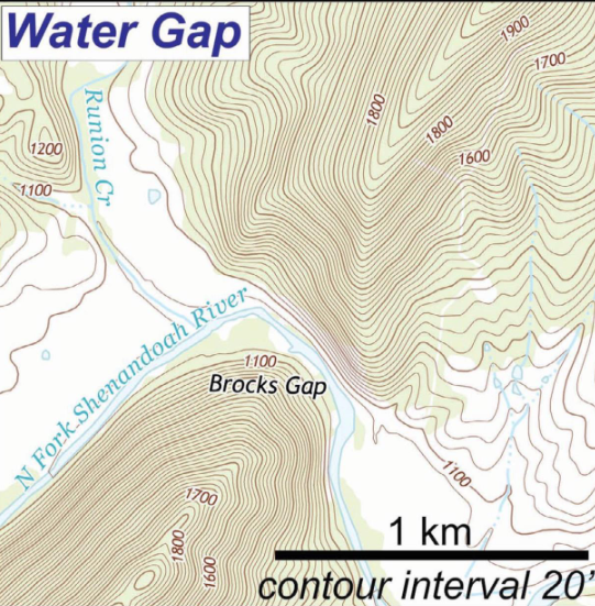
Water Gap

Gap through a ridge with stream cutting the topography of the ridge

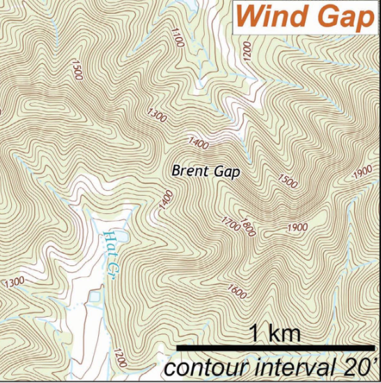
Wind Gap & Theories

Gap through a ridge but with no stream cutting through it

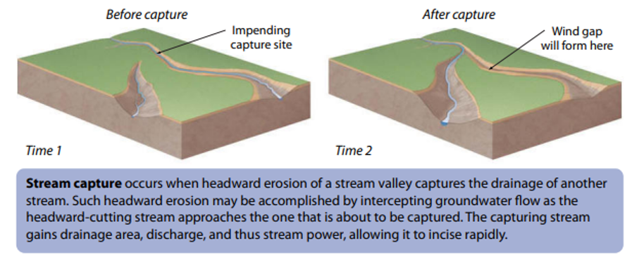
One theory suggests it used to be a water gap with the stream diverted by stream capture and headward erosion, but this is supposedly bogus

• Rockfish water gap (now wind gap) should’ve shown watershed crossing from Shenandoah to Blue Ridge, but no fluvial deposition to prove this

• Additionally, elevation differences across wind gap don’t seem feasible to have a stream at.

• No real good other explanation, however

Stream Capture Cont.

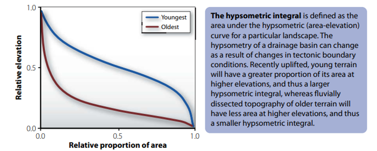
Hypsometry

The relative proportion of elevation to contributing drainage area in a drainage basin

• Young —> Larger hypsometric integral and more contributing area at higher elevations

• Old —> Smaller hypsometric integral and less contributing area at higher elevations

Main knickpoint-forming causes

• Rising base level

• Tectonic uplift

  • Also tectonic processes such as faulting

• Different lithology

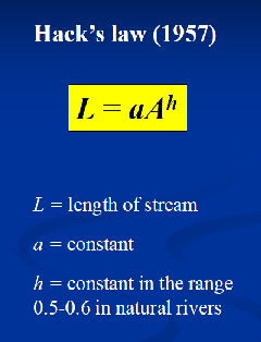
Hack’s Law

As the distance along a stream increases, so does the drainage area and therefore discharge

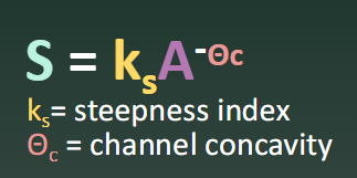
Fluvial Power Law

Generally, as slope increases, the drainage area of a stream decreases and vice versa.

Slope of a channel varies as an inverse power law of drainage basin area modified by steepness index (uplift and precipitation effects) and concavity (process domain characteristics)

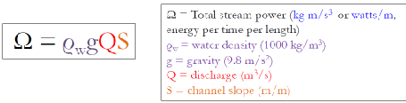
Stream Power

Stream Power = (gravity)(water density)(discharge)(slope)

Unit stream power can be found by dividing this by width of stream

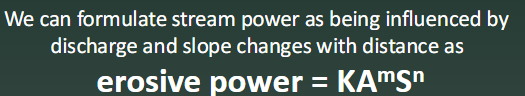
Stream Power Reformulated (Erosive Power)

Discharge changes in accordance with drainage area, so drainage area is substituted for discharge in the stream power equation.

K = Constant based on rock type, precipitation, et.

A = Drainage Area

S = Slope

m = Relative importance of drainage area

n = Relative importance of slope

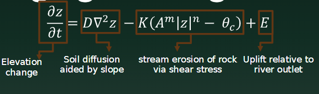
Elevation Change Equation (NEW; DIRECTLY LINKED TO LEARNING OBJECTIVE)

Elevation Change = Soil Diffusion - Stream erosion + Uplift

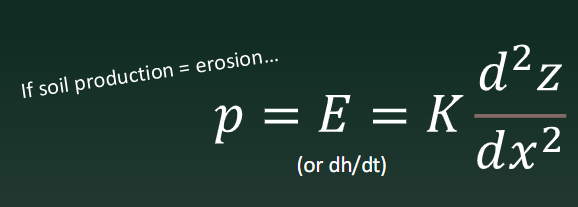
Diffusivity Equation (when soil production balances erosion)

Erosion rate = (Diffusivity)(Curvature)

Used to model hillslopes with majority diffusive processes

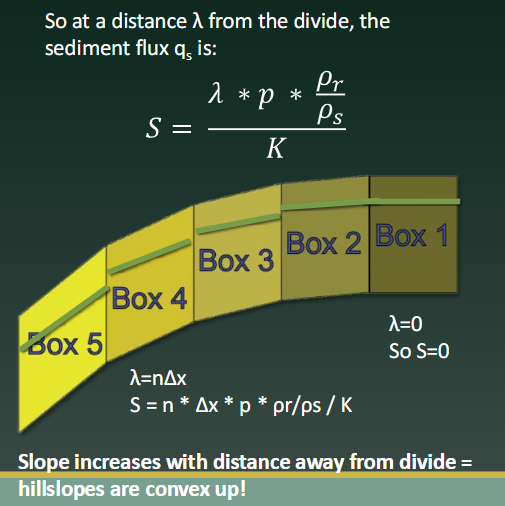
Why are hillslopes convex?

Assuming constant soil height, q = KS, where soil flux increases proportionally with slope, and the idea of soil boxes with accumulating flux

As your distance from the ridge increases and therefore your accumulated flux, the slope of the hillslope must increase, steepening it in such a way that the hillslope must be convex shaped

Why are channels concave?

According to Hack’s Law, as distance along a stream increases, so does drainage area/discharge, while fluvial power law states slope decreases as drainage area increases.

Thus, as length across a stream increases, slope decreases, creating a concave profile

Hydraulic Radius

Area of flow / Wetted perimeter

Effects of Hydraulic Radius on Various Components

Higher hydraulic radius = Higher shear stress on bed

• Streambed stress equation

Higher hydraulic radius = Faster flow velocity

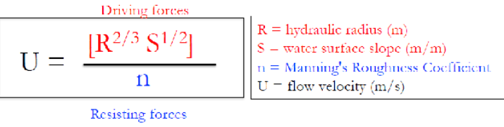
• Manning’s Equation

Manning’s Equation

Flow velocity = (Hydraulic radius)^0.66(Water-surface slope)^0.5 / Manning’s Roughness Coefficient

Hydraulic Radius is more important than slope

For hydraulic radius, a larger wetted perimeter with the same area = lower velocity of water

Manning’s Roughness Coefficient

Determines roughness of stream; empirical constant you plug into Manning’s Equation

I suppose this represents the resistance the streambed acts on the water passing over it

Darcy’s Law

Q = KA(Δh/L)

Discharge = (Hydraulic Conductivity)(Cross-Sectional Area)(Slope)

For subsurface flow

Hillslope Hydrology Review:

• Horton Overland Flow

• Saturated Overland Flow

• Shallow Subsurface Storm Flow

Shallow Subsurface Storm Flow:

• Infiltration capacity > Rainfall rate

• Subsurface flow that does not breach the surface

Horton Overland Flow:

• Infiltration capacity < Rainfall rate

• Subsurface is not saturated; water all flows above land due to lack of permeability

• Why deserts flood so fast and dramatically; desert pavement

Saturated Overland Flow:

• Infiltration capacity > Rainfall rate

• Subsurface is saturated; overland flow as soil is full

• In concurrence with shallow subsurface storm flow

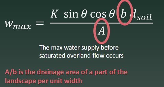
Max Amount of Water before Overland Flow (wmax)

ksin(θ)cos(θ) = Linear shallow subsurface flow discharge

• k is hydraulic conductivity from Darcy’s Law

• kcos(θ) represents what leaves on overland flow (?)

• sin(θ) represents what is going down through the soil (?)

bd_soil = Dimensions of the soil; makes SSF 3D

A = Drainage area

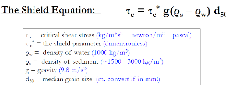
Shields Equation

• Difference in grain density and water density

• Slope

• Shield’s Parameter

• D50 of the Sediment (median grain size)

AN INCREASE OF ANY OF THESE INCREASES SHEAR STRESS NEEDED TO MOVE PARTICLES ON STREAMBED (or… at least the median sized particle)

Initial Conditions

The setup of a model before the experiment begins

• Ex. Starting elevation/volume

• Ex. Shape of sand in a hillslope tub (Lab 6 example)

Boundary Conditions

The rules that govern what happens at the edges of a model

• Ex. The edges of a box or the edges of a graph model, holding sediment in

• Minimum and maximum heights on edges. etc.

Time Step

For most model, a time step is essential to processing change over time in a model

• Ex. New data every 5 minutes, etc.

Landscape Evolution Factors

Landscape evolution:

o   Tectonics

o   Climate

o   Topography

o   Geology

o   Biology

o   Similar to ClORPT

Three Types of Models

• Conceptual models

• Physical models

  • Like our hillslope box

• Mathematical models (which can be translated to computer models)

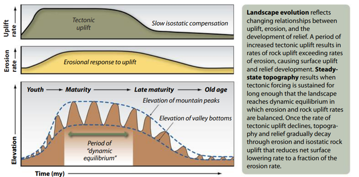
Conceptual — Dynamic equilibrium

Landscape characteristics vary over time around a central tendency

• Ex. Erosion and uplift rates are about equal; mature landscape

Mathematical — Transport Laws

Generalized mathematical expressions formalizing relationships between sediment movement and key governing variables

Mathematical transport law for diffusive processes

Sediment discharge = (Rate Constant)(Slope)

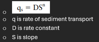
Mathematical transport law for advective processes

THE SAME ONE AS EROSIVE POWER THAT WE FORMULATED IN LECTURE

Effect of Toggling Diffusion in a Digital Landscape Model

On — Less streams as they seem to fill in and diffusive processes act

Off — Much more channel dominated with few smooth hillslope formations indicative of diffusion processes