Labour Economics Papers

Angrist and Krueger (1991)

"Does Compulsory School Attendance Affect Schooling and Earnings?"

Birth date and compulsory schooling laws (age 16).

Method: natural experiment (changes of compulsory schooling laws) and an IV (quarter of birth as an instrument); also used an OLS; the IV estimate is local average treatment effect (only affected a subgroup of people); they didn’t call it LATE because they only came up with that term in 1994 (Nobel prize paper)

Why an IV? Because Mincer (1974) equation is biased (OLS).

Results: Season of birth (Q4) is related to educational attainment and earnings for non-college graduates (7-9%). No effect on college graduates, i.e., the IV truly captures the compulsory school attendance.

Why do you use an IV (2SLS)?

Ability bias (selection bias). To address problems with endogeneity (IV helps to isolate the exogenous variation in the endogenous variable). Makes the results causal!

Lochner and Monge-Naranjo (2011)

"The Nature of Credit Constraints and Human Capital"

Studies the impact of family income on college attendance (omitted variable), in addition to ability.

Method: Simulation, not empirical: 1. simple two-period intertemporal model (baseline) 2. multi-period life cycle model (expanded analysis).

Both models allow for borrowing from the government (GLS) and private credit. There are constraints on borrowing (maximum limit).

Results: Without government loans, the poorest students don’t go to college. GSL benefits the poorest students the most. Repayment period matters too, i.e., longer is better. Ability matters for private lending, i.e., only the smartest students get private credit.

Oreopoulos and Salvanes (2011)

"Priceless: The Nonpecuniary Benefits of Schooling"

THE TWIN STUDY! (and siblings)

Significant nonpecuniary benefits beyond financial returns.

Method: Twins as an IV. The twins are the same (same ability), so you isolate the schooling effect.

Results: Even after controlling for income, higher schooling means better social, happiness, health, etc. outcomes (non-penuciary benefits). Societal benefits, e.g., lower crime rate, are often greater than private benefits.

The results are robust and causal.

Card (1995)

"Using Geographic Variation in College Proximity to Estimate the Return to Schooling"

Geographic variation in college proximity can be used as an exogenous determinant of years of schooling.

Method: uses an IV (college proximity) and OLS as the baseline test

Results: IV estimates are 25%-60% higher than conventional OLS estimates, i.e., more accurate methodology. OLS underestimates true returns to education. Living close to a college increases your probability to get a degree, i.e., higher wages. The strongest effect is for poor families living close to a college. Thus, geographic proximity is a valid instrument for estimating returns to education. Previous studies likely underestimate the returns to education.

Swinkels (1999)

Related to Spence’s signalling model.

Low ability workers have a tendency to overeducate themselves and mimic high ability workers. However, high ability workers don’t do that and may even under-educate themselves if employers cannot recognise your ability based on education from a low ability worker. That’s known as a pooling equilibrium (important concept). It happens when you introduce hiring while in school (Weiss, 1983). A separating equilibrium reveals which worker is what type.

Weiss (1983)

"A Sorting-cum-Learning Model of Education"

Key takeaway: This paper is a critique and extension of Spence (1973) and of other papers on this topic. Adding hiring while studying creates a pooling equilibrium. Related to Swinkels (1999).

In Spence (1973), the result that there is overeducation rests on the assumption that employers don’t hire individuals while they are still in school, which is satisfied in Spence’s model (1973) and has been criticized by others (Weiss, 1983).

Weiss (1983) combines sorting and learning effects, showing that when education affects productivity (assumption different than Spence’s) and enables sorting, there may be underinvestment in education. This contrasts with pure sorting models that predict overinvestment and human capital models that predict optimal investment.

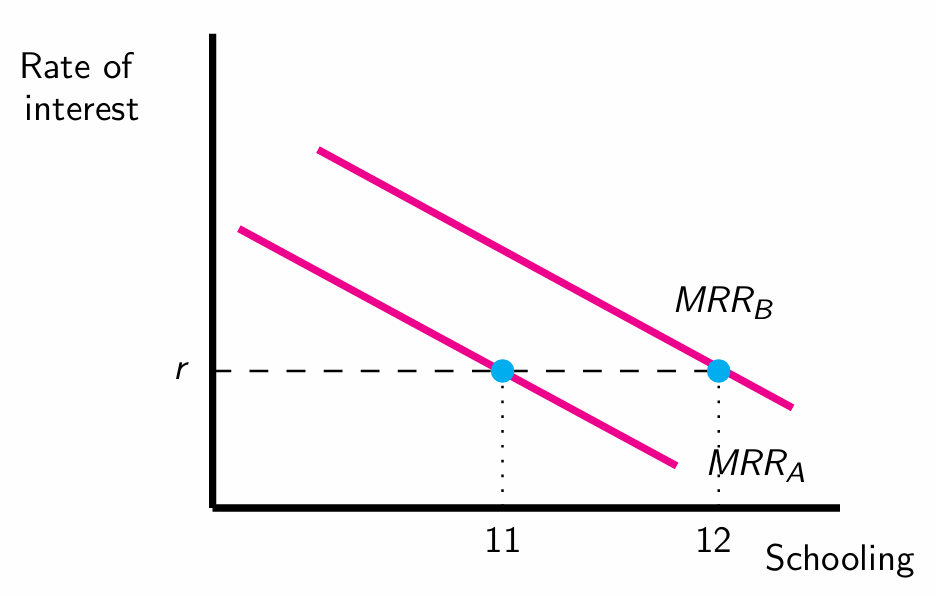
Card (2001)

Created the Basic Human Capital Model.

You either study or work. Experience affects earnings.

Optimal level of schooling depends on 1. discount rate (r) 2. ability (MRR = marginal rate of return to education)

Blundell et al. (1998)

"Estimating Labour Supply Responses Using Tax Reforms"

Captures the effect of changes in taxation on the British labour supply for women.

Method: Exogenous change in taxation affects wages. Group estimators (2 groups: high or low education), i.e., you calculate group means of hours and wages in every point in time and use a DiD. It removes all unobservable time invariant characteristics and isolates the effect. Also use an IV since simple OLS might be biased (reverse causality bias). Robust when FE are included.

Results: Higher wages mean higher labour supply through the compensated wage effect (SE or Hicksian), i.e., SE dominates the wage elasticity.

Income elasticity is dominated by the IE or Marshallian, i.e., women (with children) work less when their non-wage income (husband) is high.

Results consistent with the Basic Model.

Camerer et al. (1997)

"Labor Supply of New York City Cabdrivers: One Day at a Time"

Attempts to examine the (dynamic) Life Cycle Model, i.e., differentiates between transitory and permanent wage changes. In theory, workers should work more when wages go up (SE).

Method: OLS and IV of log hours and wages. IV uses “peer dynamics” to capture exogenous variation. Concept of income targeting, i.e., you stop once you reach certain daily income. Randomisation, i.e., taxi drivers have flexible shifts. Wages of taxi drivers are transitory, i.e., low correlation between days. Controls for weather, seasons, and special days. Considers level of experience or type of ownership, e.g., rental, owner. Mention why did he chose cab drivers?

Results: Wage elasticities are negative, i.e., taxi drivers stop working earlier on high-wage days and work more on low-wage days. The IE dominates. This violates the life cycle model.

Camerer et al. (1997) are wrong and misinterpreted the results! Farber (2005) corrects them. Target earnings hypothesis is not valid.

Farber (2005)

"Is Tomorrow Another Day? The Labor Supply of New York City Cabdrivers"

Response to Camerer et al. (1997) that proves that the life cycle model works.

Method: The Discrete-Choice Stopping Model (also known as survival time (hazard) model that uses probit. The model calculates the probability of a driver ending the shift after each trip. Considers time, wage, weather, experience, and other factors.

Results: The probability of stopping increases with time, but not with income. There is no evidence of income target or limit. Camerer et al. (1997) effect is not IE, but just the effect of fatigue (hours worked). Farber (1995) confirms the validity of the life cycle model.

Note that Farber (2005) doesn’t estimate a wage elasticity of labour supply, only the probability of stopping. That would require an exogenous shift in earnings.

Fehr and Goette (2007)

"Do Workers Work More if Wages Are High? Evidence from a Randomized Field Experiment"

Focuses on the life cycle model and bike messenger in Switzerland.

Method: RCT (randomised field experiment), i.e., strong for proving causality. Control: N/A Treatment (dummy T): 25% transitory increase in commission rate for 4 weeks, then the groups switched. Analyses the effect on total revenue, total revenue per messenger, the number of shifts worked, and the effort per shift, i.e., revenue per shift. More shifts=higher effort. Higher wages=lower effort? “Will the treatment group provide more labour supply?”

Results: The treatment group always worked more hours than the control group (positive intertemporal labour supply elasticity). Consistent with the life cycle model. intertemporal SE at its finest, i.e., T worked overtime.

However, workers reduce their effort (revenue per shift) when wages are higher even though they work more shifts. Related to loss aversion and preferences, i.e., when you reach your target, MU of extra income decreases, so you reduce effort.

Policy implication is that it’s important to consider effort when designing optimal wage policy. Higher wages may not increase productivity but only increase output.

Bloom et al. (2009)

"Fertility, Female Labor Force Participation, and the Demographic Dividend"

The effect of fertility on female labour supply.

Explores the relationship between fertility rates and female labor force participation, and how changes in fertility can influence economic growth through increased female labor supply.

Method: simple model of female fertility and labor supply choices, abortion legislative (abortion index) as an IV for fertility to address endogeneity, key explanatory variables: total fertility rate, urban population percentage, capital stock per working-age person, infant mortality rate, and average years of schooling for men and women; the utility function for a representative woman is defined over household consumption, leisure, and fertility, includes constraints on time allocation and consumption, e.g., work, leisure, and childcare.

Results: A country will gain (increase in GDP per capita income) when women start having less kids since labour market participation goes up. Yes, having kids ruins your career and earnings. Higher fertility rates significantly reduce female labor force participation. Each birth reduces total labor supply by about 1.9 years per woman during her reproductive life. Not having kids, i.e., reduction in fertility, has a positive impact on your earnings. More educated women work more. Using the abortion index is a good IV!

Autor, Katz and Krueger (1998)

"Computing Inequality: Have Computers Changed the Labor Market?"

Non-essential paper. May be used as additional evidence when paired with other SBTC papers.

Examines the effect of skill-biased technological change (SBTC) as measured by computerisation on wage differences.

Results: Finds capital-skill complementarity, where computer technology and other forms of capital are complements to more-skilled workers. The fastest growing industries (tech) also employed the greatest share of college-educated workers and didn’t hire high school-educated workers. Wages in these industries were also higher, which increased wage inequality.

Acemoglu (1998)

"Why Do New Technologies Complement Skills? Directed Technical Change and Wage Inequality"

Explores the relationship between skill-biased technological change (SBTC) and wage inequality, particularly focusing on why new technologies tend to complement skilled labor.

Method: Acemoglu develops a model where technological change is directed by the relative supply of skilled and unskilled workers. The model assumes that new technologies (either high-end or industrial) are more profitable when they complement the more abundant type of labor. Quasi-Heckscher-Ohlin model. 2 types of workers and 2 types of technology.

Results: Introduces the notion of Direct Technological Change, i.e., the abundant sector grows, innovates faster, and encourages other people to get educated. This reduces the skill premium in the short run, but innovation (STBC) increases it again. Creates wage inequality.

Relevancy: Papers by Krusell et al. (2000), Galor and Moav (2000), and Garicano and Rossi-Hansberg (2004) try to explain why this phenomenon happened in the first place using 3 different approaches.

Krusell et al. (2000)

"Capital-Skill Complementarity and Inequality: A Macroeconomic Analysis"

Extension of previous studies that concluded that the SBTC is the main reason for the skill premium (and wage inequality), e.g., Acemoglu (1998).

This paper aims to understand the role of that capital-skill complementarity in explaining the changes in the skill premium.

Method: four-factor aggregate production function (capital equipment, capital structures, skilled labour, unskilled labour) that allows for different elasticities of substitution among the factors. Incorporates capital-skill complementarity, i.e., the elasticity of substitution between capital equipment and unskilled labor is higher than that between capital equipment and skilled labor. Thus, growth in capital increases MPL (productivity). Productivity=wages, so skill premium. Low-skilled workers don’t improve MPL, it actually goes down (low adaptibility). Statistical method is a two-step simulated pseudo-maximum likelihood (SPML) estimator.

Results: 1. The relative growth of skilled labor input reduces the skill premium. 2. Improvements in the efficiency of skilled labor relative to unskilled labor can increase the skill premium if the elasticity of substitution between the two types of labor is greater than one. 3. Faster growth in capital equipment tends to increase the skill premium as it increases the relative demand for skilled labor.

With capital-skill complementarity, changes in inputs cause wage inequality, i.e., skill premium

Solution: Better education and training reduce inequality. Restricting immigration does not help.

Galor and Moav (2000)

"Ability-Biased Technological Transition, Wage Inequality, and Economic Growth"

Highly educated workers find it cheaper and easier to adopt to new technology.

Method: developed an endogenous growth model of a small production economy (with both exo/endogenous ability-biased technological change and heterogenous labour force as input). High-skilled individuals have a comparative advantage in adopting new technology (skill premium; ability) and they also improve it.

Results: Positive feedback loop. 1. An increase in technology raises the rate of return to ability for the high-skilled, but a temporary decline in wages of the low-skilled 2. That promotes education, i.e., higher supply of educated workers 3. An increase in human capital increases the rate of technological change 4. The loop repeats and creates perpetual growth (and creates wage inequality and promotes education). Overall, the skill premium is driven by ability.

Garicano and Rossi-Hansberg (2004)

"Inequality and the Organization of Knowledge"

Technology changes the organisational structure within firms, which favours the skilled workers (wage inequality).

Method: model of production that sorts workers into teams (equilibrium) and considers the impact of a reduction in the cost of communicating knowledge (information is cheap these days). Teams are different in ability.

Results: Technology change benefits the high-skilled workers the most. The reduction in communication costs (access to information) reduces inequality among workers, but more inequality among managers, i.e., some managers can leverage technology better than others.

Manning (2021) and Manning (2001)

Manning (2021): "Monopsony in Labor Markets: A Review"

A literature review of other papers on market structure.

Evidence that employers have considerable monopsony power in labour markets.

When answering a question about market structure, refer to Datta (2024). It’s a better paper.

Dal Bo, Finan and Rossi (2013). Randomised wage offerings of Mexican public sector to see how applicants respond. Results: Application-wage elasticity of 2, i.e., very responsive & applies more people. Limitation: Public sector may not be a good representation of a competitive market.

Summary of 3 other papers…

Generally, the results suggest labour markets exhibit some monopsony power, i.e., no perfect competition.

Manning (2001) as a standalone paper. Steady state of employment (Labour Supply) = Recruiting rate / Separation rate OR L(w)=R(w)/S(w). Thus, εLW = εRW −εSW (all elasticities). Because of Manning (2001), many papers aim to just estimate one elasticity (assume they are equal; εRW = εSW), but that’s questionable.

Key point: The fact that there’s monopsony can be exploited and help in explaining why minimum wages do not cause unemployment and work in the opposite direction (reducing) of monopsony power, e.g., Card and Krueger (1994), and how much can you increase the MW before it starts having a negative impact. Additionally, the monopsony condition can be used to explain the effect of immigration and anti-trust on labour elasticity and wages.

Datta (2024) Monopsony (market structure)

"The Measure of Monopsony: The Labour Supply Elasticity to the Firm and its Constituents"

(Weather Spoons) —> RANDOM LARGE FIRM IN THE UK

The importance of understanding monopsony power in the labour market (labour supply elasticity to the firm = recruitment + separation elasticity).

Method: Uses a tripple-difference estimator. Estimates recruitment (willingness to join at a given wage) and separation (willingness to stay) elasticity for a firm. 2 novel instruments (IV) as sources of exogenous variation: 1. Living Wage Floor, i.e., a location-specific wage floor that affects a small number of workers in an area but is binding only for the firm in that location. 2. Annual Leave Wage Saliency, i.e., variation in the posted wage due to the inclusion of annual leave top-up in the advertised wage, induced by idiosyncrasies in the firm's HR department.

Results: Labour markets exhibit some monopsony power (not perfect competition), i.e., wage markdown of 18% from MPL (so wages don’t equal productivity). Recruitment elasticity is 2x greater than separation elasticity, i.e., additional frictions for existing workers, less likely to leave. Must use both elasticities to estimate monopsony power (labour supply elasticity). Using completed hires (some are rejected) and applicants (some don’t take the job due to the low wage) leads to bias (downward & upward), i.e., not a good measure of elasticity. Very common bias in other studies. The paper calculates the true number of recruits via detailed firm data, i.e., people that actually want to work there. No evidence of anticipatory effects or local spillovers.

Card and Krueger (1994)

"Minimum Wages and Employment: A Case Study of the Fast-Food Industry in New Jersey and Pennsylvania"

The impact of minimum wage increases (during a recession) on employment in the fast-food industry.

Method: Exogenous increase of the minimum wage in New Jersey. Fast-food industry because: homogenous, many minimum wage workers (similar to a perfectly competitive market). Natural experiment. Control: FF workers in eastern Pennsylvania (border state) Treatment: FF workers in New Jersey. DiD on employment changes. Data via phone survey before & after the increase. Other industries shouldn’t be affected by the increase, i.e., the study compares low-wage vs high-wage stores. All natural experiments exploit the parallel trend assumption (same results in the absence of T).

Results: No significant job losses or price increases in NJ after the MW increase. This violates the classical/neoclassical view (standard competitive model), i.e., unemployment and prices should go up. Monopsony (checked via bonuses; FF resembles monopsonies) and job-search model also fail to explain it, i.e., they don’t know, and economists are divided. In theory, MW change can raise employment by offsetting the monopsony power. Prices are passed onto customers.

Limitations: The parallel trend may not hold due to 1. spillovers (travelling across the border for work) 2. different economic and geographic conditions in the two states (urban vs rural, recession). Can be checked by a placebo test or 3DiD.

Machin et al. (2003)

"Where the Minimum Wage Bites Hard: Introduction of Minimum Wages to a Low Wage Sector"

The effects of the introduction of a National Minimum Wage (NMW) in the United Kingdom on the residential care homes industry, a heavily affected low-wage sector. No MW in the UK before 1999.

Method: event study using DiD and an IV of wage gap; just without a control group, i.e., the entire UK was affected. Residential care homes selected for the same reason as fast-food workers in Card and Krueger (1994), i.e., MW workers, no unions, homogenous products. Prices cannot be passed onto customers, i.e., we should see unemployment. Tests for parallel trends by using earlier period when there’s no MW as a placebo for wage and employment.

Results: Wages rose significantly and the MW reduced wage inequality. Only a small negative effect on employment. No evidence of price or productivity increases. A firm with 10% more workers paid less than upcoming MW see 1.5% faster wage growth, i.e., these workers benefited the most. Policy implication is that the poorest workers benefit the most from MW increases. Downside: The results may not be generalised for the whole UK (very specific sector).

What is the "wage gap" (IV) variable?

The wage gap is calculated for each firm and represents the average increase in wages needed to bring all workers who are paid below the mandated minimum wage up to that minimum wage level (after the introduction of the new minimum wage).

The wage gap analysis demonstrates that the introduction of the minimum wage had a significant impact on the wage structure in the care home sector. It effectively raised the wages of the lowest-paid workers, reducing wage inequality within the sector. The findings suggest that the minimum wage "bit hard" in this sector, meaning it had a substantial effect on wages and wage distribution.

Borjas (2003)

"The Labor Demand Curve Is Downward Sloping: Reexamining the Impact of Immigration on the Labor Market"

Different than the area approach (Card 1990) for estimating the effect of immigration.

Develops a new approach for estimating the labor market impact of immigration by exploiting this variation in supply shifts across education-experience groups at a national level.

Key assumption: Workers with the same education, but different levels of experience are not perfect substitutes.

Method: linear regression with some interaction terms (education, experience, time).

Compares the effect by skills and wages on a national level, not only a regional level. Considers different levels of education and years of experience (cells).

We expect fall in relative wages of groups with higher penetration of immigrants.

Results: A 10% increase in immigrant share reduces native wages by 3-4%. Yes, immigrants reduce wages for the natives.

Limitations: Does not tackle endogeneity issues! Serious issue. For the results to be causal, we must assume that immigrants and natives are perfect substitutes with their cell.

Critique: Wages determined by occupation, not skill.

Card (1990)

"The Impact of the Mariel Boatlift on the Miami Labor Market"

Cuban immigrants coming to Miami. Focusing on the wages and unemployment rates of the low-skilled workers.

Method: natural experiment (exogenous shock). Data on labour market outcomes (wages, etc.) of different ethnic groups before & after they arrived. DiD approach to compare Miami to other US cities and their ethnic groups, e.g., Atlanta, Houston.

Limitations: 1. The test isn’t very powerful due to limited pre-event data. For a strong natural experiment, you need good pre- & after data. 2. Assumes that business cycles affect everyone (and all cities) equally. 3. Endogeneity, i.e., out-migration of native residents, which can reduce wages. The study doesn’t account for it, but it does not invalidate the study. One criticism of the area approach.

Results: No significant impact on wages or unemployment in Miami, i.e., the labour market is well-setup to absorb Cuban immigrants.

Chiswick (1978)

"The Effect of Americanization on the Earnings of Foreign-born Men"

Compares the earnings of foreign-born men with those of native-born men and explores how various factors, such as schooling, labor market experience, and time spent in the United States, affect earnings.

Method: Mincer-style regression on earnings (earnings upon arrival and years spent in the country)

Results: Immigrants earn 16% less than natives at arrival. After 10-15 years, foreign born men earn more than the natives (positive assimilation effects). Happens due to positive self-selection, i.e., those that immigrate are better. Earnings vary significantly by country of origin. Immigrants from Mexico, Cuba, and Asia/Africa tend to have lower earnings compared to those from English-speaking developed countries.

Borjas (1985)

Builds on Chiswick (1978) but considers cohort effects.

Method: Chiswick (1978) only estimated a single cross-section (likely biased). Borjas (1985) estimates 4 cross-sections (4 cohorts). Those that immigrate earlier are different, i.e., higher in ability.

Results: Almost all results suggest “decline in the quality of immigrants over time.” Those that came earlier have higher earnings.

Limitations: Out-migration, i.e., if you are not doing well, you leave. To solve this, you must consider only migrants that stay in the US.

Gibson et al. (2018)

"The Long-Term Impacts of International Migration: Evidence from a Lottery"

Tonga lottery. The impact of migration on migrants.

Method: natural experiment, but still local average treatment effect, i.e., self-selection into ballot and still choice to move. Randomisation is provided by the lottery (randomly selected to migrate via a lottery). Control: unsuccessful applicants Treatment: winners and those that migrated (over 80% of winners migrated). Data collected through face-to-face interviews, lab-in-the-field, and long surveys over multiple years (small sample overall). Focus on the experimental design when explaining this study!

Results: Wages doubled. Increase in education (studying). Generally strong positive impacts. Limited impact on extended family (except receiving more personal remittances). Migrants 30% more likely to be employed

Limitations: Cannot be generalised to different countries or individuals due to heterogeneity (individual and country differences).

Neal and Johnson (1996)

"The Role of Premarket Factors in Black-White Wage Differences"

The key idea is to understand how to spot discrimination using empirical studies.

The paper examines the role of premarket factors, e.g., family environment, access to education, and other differences, in black-white wage differences, particularly focusing on the impact of skill differences.

Limitations: Estimation results are highly sensitive to the inclusion of controls, especially skills and education. No occupation controls. Note that these controls can be biased, i.e., education is pre-determined by discrimination (conditional mean independence assumption). Challenging to isolate discrimination from other factors. Empirically, if the gap persists even after including all the controls, discrimination is present.

Method: Regression models of log wage rates on age, ethnic or racial group dummies, and the AFQT test score, i.e., multiple controls.

Results: The AFQT test score explains between 75% to almost 100% of the wage gap between the white and black workers. However, these test scores are determined by family background and level of education and thus, the study highlights societal and economic disparities.

No evidence of discrimination, i.e., it is explained by family and school environment. Discrimination in other areas, e.g., labour market, is not tested, so it cannot be ruled out.

O’Neil and O’Neil (2006)

Gender gap and discrimination.

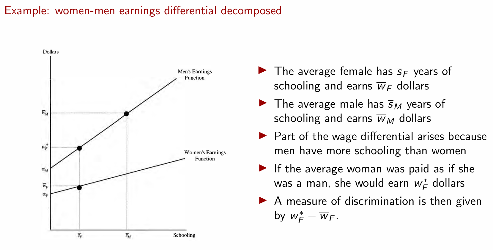
Method: Uses the Blidner-Oaxaca method (decomposition method). Estimates separate wage equations for the different groups (one for men, one for women). Identifies what can be explained by individual characteristics, what’s left unexplained is due to discrimination.

Blinder-Oaxaca method

1. Estimate 2 separate wage regressions. 2. Subtract them. Some parts can be explained, some of them cannot and that’s evidence of discrimination. 3. Decomposition columns shows discrimination (total unexplained by the model).

Results: The unexplained component shows that there is discrimination. Results show that women are discriminated against men.

Limitations: Causal interpretation requires certain assumptions to hold. 1. Conditional mean independence assumption 2. Existence of common support (same effect on both groups) 3. Invariance of the conditional distributions (assumes that the world is not a zero-sum game). There is also selection bias (only those that work). Bad controls. Also, possible omitted variable bias.

Goldin and Rouse (2000)

"Orchestrating Impartiality: The Impact of 'Blind' Auditions on Female Musicians"

Audit studies can be used to spot discrimination.

Blind auditions (using a screen) to conceal the candidate’s identity. Sex-biased hiring, i.e., common belief that female musicians are not as good as their male counterparts. The aim is to increase the number of women in orchestras (currently underrepresented).

Method: regression with dummies for female and blind audition (and other controls). Treatment effect is Female X Blind. Measures the probability of a woman advancing to further rounds or getting hired. We want to see women getting to further rounds when blind to prove discrimination.

Results: Yes, there is discrimination. Positive treatment effect across most specifications. 12% increase for females in earlier rounds. However, later rounds are noisy (makes sense, final rounds are all about the winner takes all).

Limitations of audit studies: 1. Job applications are not sent at random, i.e., the role of networking. 2. Only focuses on entry-level roles; how about more skilled jobs? 3. Just binary outcomes, i.e., little insight

Bertrand and Mullainathan (2004)

"Are Emily and Greg More Employable than Lakisha and Jamal?

Investigates racial discrimination in the labor market through a field experiment, i.e., sending identical CVs but with different names.

Method: field experiment via sending fictitious CVs. Randomisation of names, i.e., either African American or white names. 2 categories of CVs: 1. high-quality candidates, e.g., better education and more experience 2. low-quality candidates. CVs were identical except the names and addresses, e.g., Boston < New York. They tracked interview call-backs.

Results: White-sounding names received 50% more callbacks for interviews compared to those with African American-sounding names. The racial gap consistent across cities and job categories, i.e., widespread issue. "Equal Opportunity Employer" did not significantly reduce the racial gap in callback rates. Therefore, racial discrimination still prominent in the US. There’s a need for better policies to tackle it. 1. Legal action 2. Focus on pre-market factors, e.g., non-biased education 3. Intergroup contact to reduce racism 4. Debiasing training

Same limitations as for audit studies, e.g., Goldin and Rouse’s (2000) blind auditions

Doleac & Stein (2013)

Results: Black sellers receiver fewer and lower offers than white sellers, especially in thin markets. Similar magnitudes for black and tattooed sellers vs white sellers.

Mechanisms: Evidence discrimination decreases in thicker markets, as predicted by Becker. Discrimination is higher in more racially “isolated”, suggesting a role for group identity. Consistent with statistical discrimination through profiling.

Datta (2024) ZHCs

"Why do flexible work arrangements exist?"

Analyses how firms respond to (demand) shocks, e.g., workers leaving or getting sick, seasonal demand, using ZHCs (zero-hour contracts). Focuses on the demand side. The examined firm has many workers with zero-hour contracts.

Method: regression analysis, i.e., when a worker calls in sicks, how many ZHCs workers are called in? 6 similar equations: 1. different skills between ZHCs and permanent workers 2. allows for substitutability, i.e., ZHCs workers are amazing at everything. And then, Eq. 1-2. is when they are absent and eq. 3-4. when they permanently quit. Eq. 5-6. is about demand effect of weather on ZHCs, i.e., I hire more workers when it’s hot. A firm has a reserve of ZHC workers that they can call when they need them due (demand) shocks, e.g., busy Friday, absent workers, or many people quitting at once. Seasonality in retail or restaurant industry.

Results: Complicated table! 15% means that for every 8 days of absence, I hire 1 full day of ZHC worker. Goes up to 30% (2 days) when they are substitutable. Yes, the firms are using ZHC workers to respond to short-term absence of permanent workers. When workers permanently leave, I use a ZHC worker for 3-4 months before I hire someone, i.e., delays hiring and no need to hire right away. Note that ZHC workers have higher turnover and may not come. Eq. 5-6. focuses on the temperature variation (proxy for seasonality) on the demand for ZHC workers. Yes, temperature has an effect on ZHCs, i.e., I hire more ZHCs in summer (seasonality). Note that it’s hard to force them to come to work.

Datta et al. (2019) ZHCs + MWs

"Zero-hours contracts and labour market policy"

Have higher minimum wages increased use of ZHCs? Maybe using ZHC workers may be cheaper, because you can clock people off (not legal, but happens).

Method: DiD specification; used the exogenous minimum wage increase in the UK as a natural experiment (before & after the increase of MW); the pre-period test is a placebo; focuses on the care industry; assumes the parallel trend assumption and it holds (IMPORTANT! All DiD studies assume this).

Results: YES, firms buffer the wage cost shock induced by increasing ZHCs. Further research is needed to see whether the effect stabilises. Wages increased rapidly for both care homes and personal care after MW change (~7%). Makes sense because all our workers get MW. Care home ZHCs slightly increased. Domiciliary care (personal care) ZHCs significantly (~6%).

Limitations: Cannot be generalised to other sectors.

Mas and Pallais (2017)

"Valuing Alternative Work Arrangements"

Investigates how workers value different types of work arrangements, e.g., flexible scheduling, working from home, and irregular schedules.

Method: natural experiment of observing real-life decision, i.e., willingness to pay/sacrifice for flexibility (real hiring experiment with choices). Baseline job (controI): 40 hours/week; 9to5 (standard job). Treatment: choice given to applicants, e.g., flexible schedule, more/less hours, WFH. Uses a maximum likelihood logit model to estimate the WTP distribution and a breakpoint model to account for mass points in the WTP distribution. The model included corrections for inattention, i.e., questions in a survey.

Results: Most workers did not value flexible scheduling, but the top 25 percent of workers were willing to give up a significant portion of their wages for this flexibility. Work from home is valuable (8% salary reduction). People don’t like unpredictable working hours (firm’s power). Used a nationally representative survey, i.e., can be generalised. Results consistent with other studies.

Policy implications: Firms must consider heterogeneity of preferences when designing workplace policies and compensations.

Katz and Krueger (2018)

"The Rise and Nature of Alternative Work Arrangements in the United States, 1995-2015"

Investigates the trends and characteristics of alternative work arrangements in the United States over a 20-year period.

Method: survey design (64% response rate); Regressions for the log of hourly wages, log of weekly earnings, and log of hours worked on all jobs. The analysis included variables such as years of education, years of experience, race, ethnicity, gender, and controls for 22 occupations. This allowed them to assess the wage differentials and work hours associated with different types of work arrangements, controlling for personal characteristics and occupational differences.

3 ways of measuring atypical work arrangements:

1. Directly asking in surveys 2. Discrete choice field or natural experiments 3. Discrete choice experiments from hypothetical “vignettes” in survey. Overall, it’s hard to measure them anyway.

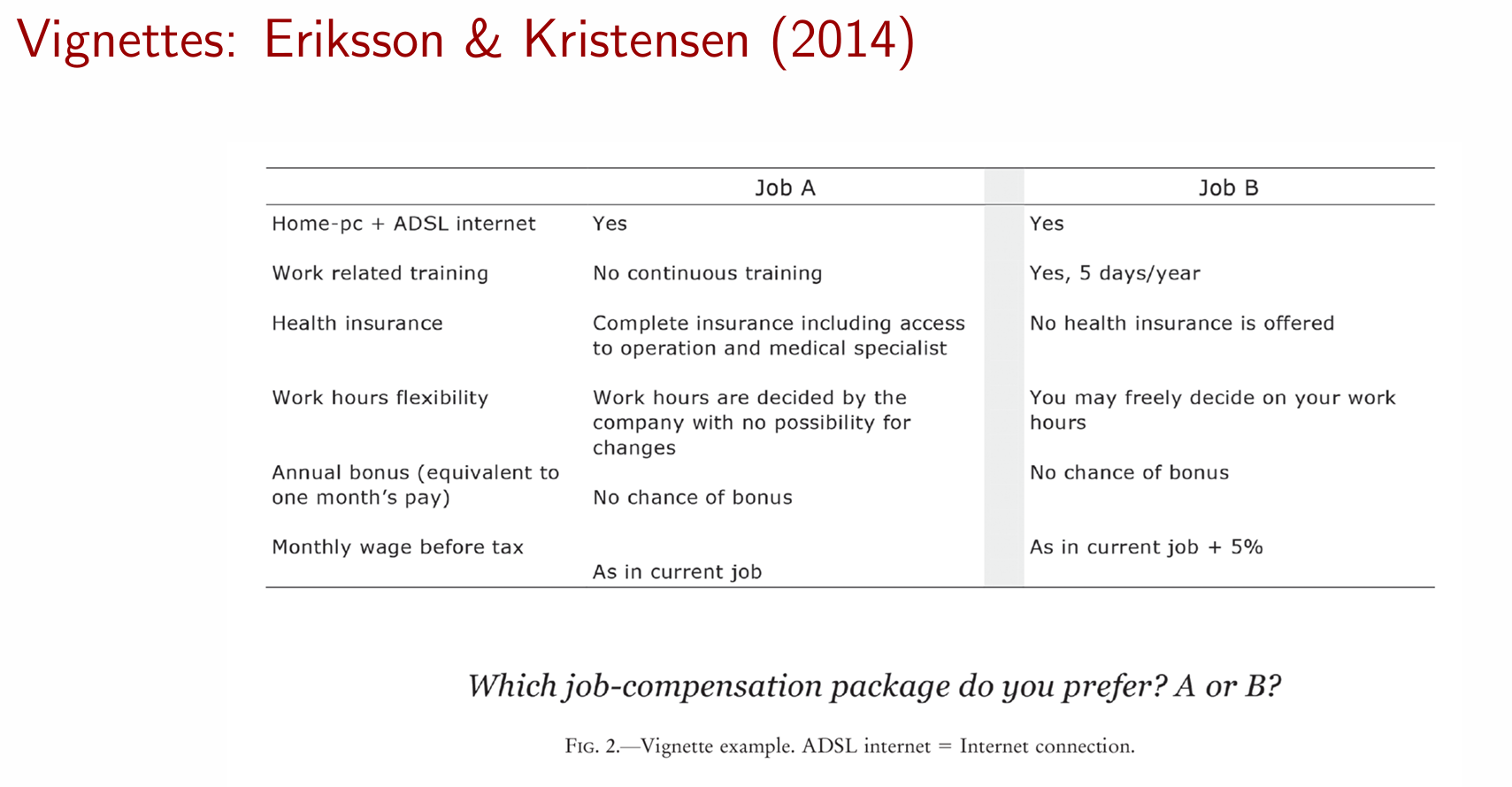
Vignette studies

Eriksson and Kristensen (2014) and Datta (2019).

Eriksson and Kristensen (2014): Use hypothetical vignettes in survey to explore trade-off between wages and extra perks/ benefits. Danish labour market. Discrete choice between two job packages A and B. Repeated 7 times for each survey respondent.

Definition: Vignette studies involve presenting participants with carefully constructed scenarios, or "vignettes," that describe situations, individuals, or events. Participants are then asked to respond to questions based on these scenarios. Vignette studies have less bias and allow for more complex scenarios/questions. Surveys are just questions without any context.

Datta (2019)

Vignette study. You are given 2 choices, pick one.

Use hypothetical vignettes in survey to explore trade-off between wages and characteristics associated with atypical work arrangements. Worker’s preferences, essentially. UK and US labour market. Similar approach to Eriksson & Kristensen (2014).

Data: From an internet-based survey, targets working-age people in the US and UK. Vignette survey design (more serious than a regular survey).

Mixed logic model.

Results: 1. Traditional employer-employee relationships is the most valued (WTP = willingness to pay, i.e., worth 50% of wage), i.e., people don’t like not being full time employes (contractors) 2. Sick pay and holiday are the second most valuable (worth 30% of wage). 3. Flexibility and location, but that’s smaller (10-20%). Also, different groups of people value different thing! —> Heterogeneity of choice.