Lvl 2: Fixed Income

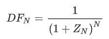
Discount factor

Zn = YTM

spot curve vs forward curve

• when the spot curve slopes upward, the forward curve will lie above the spot curve

• when the spot curve slopes downward, the forward curve will lie below the spot curve - economic slowdown

swap rate

rate for the fixed leg of an interest rate swap

govt spot curve vs swap rate curve

• depends on the interest rate exposure profile of the institution (wholesale banks hedge with swaps - swap; retails banks - govt spot)

swap spread

spread paid by the fixed-rate payer of an interest rate swap over the rate of the “on-the-run” govt security

unbiased/pure expectations theory

• forward rate is an unbiased predictor of the future spot rate

• consistent with the assumption of risk neutrality - investor unaffected by uncertainty

local expectations theory

• expected return for every bond over short periods is the risk-free rate

• No-arbitrage condition

• requires that risk premiums be nonexistent for very short holding periods, no such restrictions are placed on longer-term investments

Liquidity Preference Theory

• liquidity premiums exist to compensate investors for the added interest rate risk they face when lending long term

• upward-sloping yield curve

• downward-sloping yield curve - an expectation of deflation

Segmented Markets Theory

• allows for lender and borrower preferences to influence the shape of the yield curve.

• yield of securities of a particular maturity is determined entirely by the supply and demand for funds of that particular maturity

Preferred Habitat Theory

• strong preferences for particular maturities - does not assert that yields at different maturities are determined independently of each other

• if the expected additional returns to be gained become large enough, institutions will be willing to deviate from their preferred maturities or habitats

• notion that agents and institutions will accept additional risk in return for additional expected returns

if future spot rates lower than current forward rates

• spot < forward: purchase the bond since it is likely undervalued.

• spot > forward: short the bond likely overvalued; return < rfr

value additivity

value of the whole equals the sum of the values of the parts

• when value additivity does not hold - arbitrage profits are possible

dominance

• financial asset with a risk-free payoff in the future must have a positive price today

Binomial interest rate tree: i_H

i_1,H = i_1,Le^2σ,

i_2,HH = i_2,LL(e^4σ)

Monte Carlo method

• when a security’s cash flows are path dependent

• Interest rate paths are generated on the basis of some probability distribution and a volatility assumption, and the model is fit to the current benchmark term structure of interest rates

• A constant is added to all interest rates on all paths such that the average present value for each benchmark bond equals its market value - drift term

• implementing upper and lower bounds- mean reversion

• More paths increase the accuracy of the estimate in a statistical sense, but this does not mean the model is closer to the true fundamental value of the security.

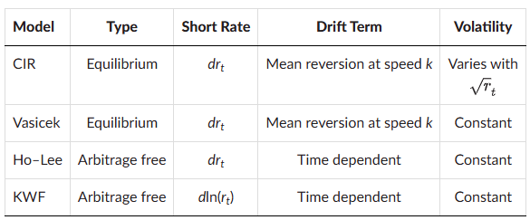
Cox–Ingersoll–Ross model

• Equilibrium model - based on market prices

• assumes interest rates follow a mean-reverting process

• drift term - rt = level of rates at t; θ= long run mean; k = speed rate reverts to mean

• random component - varies as rate changes (non negative)

Vasicek model

• Equilibrium model

• includes mean reversion at speed k

• The stochastic or volatility term follows a random normal distribution for which the mean is zero and the standard deviation is 1 - can be negative

Ho-Lee model

• arbitrage-free model - based on the current term structure

• assumption is that the reference bonds are priced correctly

• allow the parameters to vary deterministically with time

• derivatives and bonds with embedded options

• drift term is time dependent

• constant volatility (same as Vasicek) - may be negative

Kalotay–Williams–Fabozzi model

• arbitrage-free model

• log of the short rate - short rate itself is distributed lognormally

• drift term time dependent

• constant volatility (same as Vasicek) - may be negative

European-style callable bond

• european - exercise the call option only once on the call date

• american - continuously callable at any time starting on the first call date

• bermuda - predetermined schedule on specified dates

sinking fund bond

requires the issuer to set aside funds over time to retire the bond issue, thus reducing credit risk

value of callable/putable bond

Value of callable bond = Value of straight bond – Value of issuer call option.

Value of putable bond = Value of straight bond + Value of investor put option.

when to call/put

call if PV > X price

put if PV < X price

factors affecting options

• call/put options increases with volatility

• call option increases with decreasing i/r; put option decreases with decreasing i/r

• call option increases with decreasing slope; put option decreases with decreasing slope

Z-spread

fixed spread over default-free benchmark yield curve - credit quality

option-adjusted spread (OAS)

constant spread that when added to all the one-period forward rates on the interest rate tree - z spread with volatility

• as i/r volatility increases, OAS for callable bond decreases

effective duration

• can be used for bonds with embedded options - unlike modified duration

• parallel shift of the benchmark yield curve

• Eff Dur for callable bond/ putable bond < Straight bond

• Eff Dur of callable bond < straight bond when i/r falls

• Eff Dur of putable bond < straight bond when i/r increases

one sided duration

• callable bond: bigger up-duration

• putable bond: bigger down-duration - when at the money more sensitive to decrease in i/r

key rate duration

sensitivity of the bond’s price to changes in specific maturities on the benchmark yield curve

• key rate duration of bonds w options depends on time to maturity & time to exercise

• callable bond w low coupon behaves like it will not be called

• putable bond w high coupon behaves like it will not be put

Effective convexity

sensitivity of duration to changes in interest rates

• callable - positive convex > turns negative when near the money, i/r declines

• putable - always positive

capped floater

• issuer option: protects the issuer against rising interest rates

• prevents the coupon rate from increasing above a specified maximum rate

Value of capped floater = Value of straight bond – Value of embedded cap.

floored floater

• prevents the coupon rate from decreasing below a specified minimum rate

• investor option - protects from declining interest rate

Value of floored floater = Value of straight bond + Value of embedded floor

convertible bond

• investor accepts lower coupon for option to convert

conversion value

Conversion value = Underlying share price × Conversion ratio.

Minimum Value of a Convertible Bond

greater of:

• conversion value

• value of underlying option free bond

market conversion premium per share

• = Market conversion price – Underlying share price,

premium over sstright value

Value of callable putable convertible bond

Value of callable putable convertible bond = Value of straight bond + Value of call option on the issuer’s stock – Value of issuer call option + Value of investor put option.

convertible bond, straight bond, underlying stock

• underlying share price < conversion price - bond exhibits bond risk/return

• underlying share price > conversion price - stock risk/return

recovery rate

percentage of the loss recovered from a bond in default

• industry

• degree of seniority

• amount of leverage in capital structure

• whether secured or collaterized

risk-neutral probability of default

the default probability that does produce a value of 100.

credit score vs credit rating

• score - retail lending market for small businesses and individuals

• rating - wholesale market for bonds issued by corporations and government entities

FICO

• 35% payment history

• 30% debt burden

• 15% length of credit history

• 10% types of credit used

• 10% recent searches

credit rating

• senior unsecured debt

• subordinated debt is then adjusted, or “notched,”

% change in bond value

Exp change in price = Duration* (change in spread: new - current)

Probability * Exp change in price

structural credit analysis model

• a company defaults on its debt if the value of its assets falls below the amount of its liabilities and that the probability of that event has the features of an option

• provide insight into the nature of credit risk but can be burdensome to implement

• determine the value of the company, its volatility, and the default barrier

reduced form credit analysis model

• default is an exogenous (external) variable that occurs randomly

• aim to explain statistically when defaults occur

• key parameter in this process is the default intensity

• inputs are observable variables, including historical data

• default intensity estimated using regression analysis on company-specific variables and macroeconomic variables

Components of corporate bond yield

spread = risk premium = tax + liquidity + credit risk

benchmark = rf rate = expected inflation + real i/r

driver of term structure of credit spreads

• credit quality - high credit rating - low spread (flat, slightly upward sloping)

• financial conditions - expectations for economic growth

• market supply and demand - heavily influenced by new bonds

• company fundamentals

• appropriate benchmark rate (off the run maturities use swap rate)

• all-in spread over benchmark (should only include senior unsecured bonds)

slope of credit spread

• Flat credit spread curves: stable expectation of default over time

• positive slope: high-quality issuer low short-term credit spreads rising with increasing maturity

• downward-sloping credit: investor expectations that the new owners will create efficiencies in the restructured organization, leading to improved future cash flow; or cyclical industry

credit analysis approach for ABS

• loan by loan - discrete, large loans, heterogeneous

• portfolio based - granular, small loans, homogeneous, portfolio changes

• statistic based - static, ST loans, granular, homogeneous

CDS

one party makes payments to the other and receives in return the promise of compensation if a third party defaults

• Compensation equal to expected recovery when credit event happens

• protection buyer - pays periodic payments

• protection seller - compensates buyer

• similar to put options

single-name CDS

• designated instrument is usually a senior unsecured obligation

• Any debt obligation issued by the borrower that is ranked equal to or higher than the reference obligation with respect to the priority of claims is covered

• buyer is short credit exposure

cheapest to deliver obligation

lowest cost but has the same seniority as the reference obligation

index CDS

• credit correlation - correlation of defaults in the index

• more correlated the defaults, the more costly it is to purchase protection for a combination of the companies

• buyer is long credit exposure

• equally weighted

• latest-created series = on the run series - roll refers to moving to on-the-run series

CDS spread

• standardized - 1% for investment grade/index, 5% for high-yield

• discrepancy remedied through upfront payment/premium - credit spread > standard = payment from buyer to seller

credit event

• unambiguous

• bankruptcy

• failure to pay

• restructuring - involuntary (forced by creditors) or coercive (forced by borrowers)

Payout amount

Choose the cheapest to deliver Recovery amount

Loss given default = 1 – Recovery rate (%).

Payout amount = LGD × Notional

Upfront payment

PV of protection leg

• LGD x POD = EL > Discount at risk free rate

PV of premium leg

• Standardized coupon payments * hazard rates > Discount at risk free rate

Upfront payment = PV (Protection leg) – PV (Premium leg).

Upfront premium ≈ (Credit spread – Fixed coupon) × Duration

Upfront premium % = 100 – Price of CDS in currency per 100 par.

Credit spread & curve

LGD in % terms x POD

• constant hazard rate will tend to flatten the credit curve

• upward curve - greater likelihood of default in later years

• downward curve - indicator of severe near term stress

• If upward sloping and will flatten - ST maturities will increase in price (buy) LT maturities will cheapen (sell)

Change in value of CDS

Profit or loss for the buyer of protection ≈ Change in spread in bps × Duration × Notional.

% Change in CDS price = Change in spread in bps × Duration

curve trade

• believes that long-term credit risk will increase relative to short-term credit risk > buy protection on long term and sell protection on short term

basis trade

difference between a company's CDS spread and excess of the company's bond yield over the market reference rate

• negative basis trade - if bond has a higher credit spread than CDS contract - buy bond, buy protection

• positive basis trade - if bond has lower credit spread than CDS contract - sell bond, sell protection

credit analysis of commercial ABS

• loan by loan - large and heterogeneous

• portfolio based - granular and homogeneous and MT/dynamic

• statistics based - granular and homogeneous and ST

cash settle vs physically settle CDS

• physical: delivery of the debt instrument in exchange for a payment by the credit protection seller of the notional amount of the contract

• cash: credit protection seller pays cash to the credit protection buyer - receive the payout + can sell the bond if the bond is worth more than the cheapest option

TED spread or Libor-OIS spread

TED

• difference between ST MRR and the yield on a Treasury bill of the same maturity

• key indicator of perceived credit and liquidity risk- banks

Libor-OIS

• difference between MRR and the overnight indexed swap (OIS) rate

• barometer of the US Treasury repurchase (or repo) market - banks

bond risk premium

the expected excess return of a default-free long-term bond less that of an equivalent short-term bond or the one-period risk-free rate.

• impacted by monetary policy - drives variance of short and intermediate term bond yields

• impacted by fiscal policy - deficits require more borrowing - yield increases

bearish flattening

• economic expansion when monetary authorities raise benchmark rates to control inflation

• ST yield increases more than LT yields

• flatter curve - purchase LT bonds, short ST bonds

bullish steepening

• recession when benchmark rate is cut to stimulate economic activity

• lowering i/r - same LT rate

• steeper curve - short LT bonds, purchase ST bonds

bullish flattening

• highly uncertain market periods

• investors flock to govt bonds - flight to quality

• yield curve flattens as long term rates fall more than st rates

• shift from bullet to barbell

Monte Carlo model

• Drift term - the expected rate path over time - constant or mean reverting

• second term - adds randomness or volatility

• Class of model - Arbitrage free (begins with assumptions about the term structure, “parameterized” - determine variables to produce bond prices that match market prices- favoured) or Equilibrium (use fundamental economic variables to describe term structure dynamics - not bound to current market prices - for dynamic applications)

Term structure model summary

G-spread

the difference between the YTM on a corporate bond and a government bond of the same maturity

upfront premium of credit default swap

Upfront premium ≈ (Credit spread – Fixed coupon) × Duration