IIoT PDF 15: Machine Learning (Slides: 20 - 50)

Definitions and short notes

Machine Learning Lifecycle - Typical Tasks [Slide 21-22]

• Specification of the objectives

• Clarification of the available data (PLC signals, sensor signals, ...), the data rate and the data sources

• Checking whether a classical algorithm is more useful, than ML

  • If yes, use a classical algorithm!!!

  • If not, carry on with the ML lifecycle
    

• Specification and implementation of the data acquisition of training data;

• Checking for historical data, if available

• Generation of training data

  • For supervised learning: also labeling the data
    

• Selection of the Machine Learning-algorithms to be tested

• Selection of the programming environment (programming languages, frameworks, etc.)

• Selection of the metrics with which the models shall be evaluated
  

• Analyzing the data; selection of the most suitable signals/features to use; specification of the data preprocessing

• Splitting the data into training and test datasets

  • For additional validation tasks, data is oftentimes split into training, validation and test dataset

• Implementation of the data preprocessing
  

• Implementation of the training for the ML algorithms and evaluation by selected metrics

  • Iterative training of the model, if possible on the basis of pre-trained models, to find the best model parameters, thereby assessing the model quality based on the results for the verification data
    

• Specification and implementation of hardware for live predictions using online data

• Implementation of the data acquisition of the online data and of the online calculation of the trained model

• Specification and implementation of the visualization or of the use of the results

• Improvement of the model in the event of new problems arise by collecting further training data and retraining

Data Science Process: Find Suitable ML algorithms [Slide: 23]

• Step 1: Analysis of the data, the problem and the constraints:

  1. Analyzing the data
     e.g.: Basic properties, Statistics, Cleaning & Augmenting, …
     

  2. Categorizing the problem
     e.g.: by input: labelled/not labelled, number of inputs, number/class/set of input groups or by output: number of outputs
     

  3. Understanding the constraints
     e.g.: data storage capacity, max. allowable prediction time, max. allowable training time
     

  4. Finding the most suitable algorithms
     e.g.: objectives reached, amount of pre-processing, accuracy, explainable, time required, scalable, complexity

Data preprocessing [Slide: 24]

ANALYSE DATA

1. Basic properties of the data

   • No. of features (enough, not enough, too many, features that do not fit)

   • No. of samples, balance of data sets (e.g. enough data of every class, too many data of one class)

   • Numerical, categorical data; nontime-series, time series, time stamps, missing data, too many duplicates, outliers in data, …
     

2. Analyzing the data
   e.g.: Summary statistics, Percentiles, Averages, Medians, Correlations, Visualizations
   

3. Cleaning the data
   e.g.: Adding missing values, Deleting values, Filtering of values (e.g. outliers)
   

4. Augmenting the data
   Increasing the training set by creating modified copies of a dataset using existing data
   

5. Adjusting the data
   e.g.: Ease interpretation, reduce redundancy & dimensionality, rescale variables (scaling / normalization), add error or other values
   

6. Splitting the data
   e.g. 80% / 20% of the data or 80% / 20% of the cases (for training / validating)
   
   
   Analyze data again after preprocessing before training!!
   

Finding the necessary features [Slide: 25-27]

Correlation Matrices

• Display the connection between different variables in a dataset, specifically between features and labels

• Can be created in python by using corr function of pandas and matshow function of matplotlib

Problems with data in example for predictive maintenance and how to deal with them (possible data preprocessing). [Slide: 28-30]

1. Irrelevant data → Delete this data

2. Non-numerical values → Convert to numerical values

3. Large value range → Scale the value range

4. Specification of the target value (class) → Make the right decision

5. Wrong values → Delete or adjust date

6. Outliers in the data → Delete or adjust date

7. Gaps in the data set → Fill gaps sensibly

8. Wrong text → Correct text (spelling, write out abbreviations, use correct expression, translate text)

Hyperparameter Optimization [Slide: 31]

Nearly all algorithms need hyperparameters for the training (e.g. for a neural network, number of layers, number of neurons for each layer, type of activation function, number of epochs, percentage of training and test data of data set, ….). Unfortunately there are no rules for the optimal hyperparameters for the training

• Research for similar applications and the use of hyperparameters in literature

• Try and error (in a structural way, e.g. by only changing one parameter at a time) and find the best values for the hyperparameters!

• Work with grid search (Automatic execution of multiple training runs for various hyperparameter values in a structured manner) or something similar.

CLASSIFICATION METRICS

Loss functions [Slide: 33]

• Show a measure of model performance.

• Used to train a machine learning model (using some kind of optimization like Gradient Descent)

CLASSIFICATION METRICS

Accuracy [Slide: 33]

> 0.7 => average model, > 0.9 => good model, bad metric in case of class imbalance

CLASSIFICATION METRICS

Precision [Slide: 33]

Higher precision => more relevant results, focused on correctness of positive predictions

CLASSIFICATION METRICS

Recall (Sensitivity) [Slide: 33]

High recall => indicates the classifier predicts the majority of the relevant results correctly, does not take into account the potential repercussions of false positives

CLASSIFICATION METRICS

F1 Score (F-measure) [Slide: 33-34]

• Indicates the reliability of a model

• Shows a strong performance in recognizing positive cases while minimizing false positives and false negatives, > 0.9 very good, 0.8 0.9 good < 0.5 Not good
  
  False Positive (Type 1 Error)
  False Negative (Type 2 Error)

CLASSIFICATION METRICS

True Positive

True Negative

False Positive

False Negative [Slide: 33-34]

• True Positive (TP):

  • The model predicts a positive case, and the actual case is also positive.

  • Example: The model predicts a patient has a disease, and the patient actually has the disease.

• True Negative (TN):

  • The model predicts a negative case, and the actual case is also negative.

  • Example: The model predicts a patient does not have a disease, and the patient actually does not have the disease.

• False Positive (FP):

  • The model predicts a positive case, but the actual case is negative.

  • Example: The model predicts a patient has a disease, but the patient actually does not have the disease. This is also called a "Type I error."

• False Negative (FN):

  • The model predicts a negative case, but the actual case is positive.

  • Example: The model predicts a patient does not have a disease, but the patient actually does have the disease. This is also called a "Type II error."

UNDERFITTING, GOOD FITTING, OVERFITTING

Underfitting (Slide: 35)

• High loss and low accuracy(targets/points are far away from the predictions)

• Bad model

UNDERFITTING, GOOD FITTING, OVERFITTING

Good fitting (Slide: 35)

Generalized model is not perfect, but close to the actual relationship

UNDERFITTING, GOOD FITTING, OVERFITTING

Overfitting (Slide: 35)

• Model has memorized the training data and is therefore super good for the training data but bad for test data

• Bad model

How to choose the right algorithm? [Slide: 37,40]

• No best method or one size which fits all

• Finding the right algorithm is partly trial and error

• Also depends on:

  • Size and type of data

  • Insights one wants to get from the data

  • How those insights will be used

What do you want to do with your data → Algorithm cheat sheet
Additional requirements:

• Accuracy

• Training time

• Linearity

• No. of parameters

• No. of features

How to choose the right algorithm? (Classifications) [Slide: 38]

1. Machine Learning

   • Supervised Learning

     • Classification

       1. Support Vector Machines

       2. Discriminant Analysis

       3. Naive Bayes

       4. Nearest Neighbor

     • Regression

       1. Linear Regression, GLO

       2. SVR, GPR

       3. Ensemble Methods

       4. Decision Trees

       5. Neural Networks
          

   • Unsupervised Learning

     1. Clustering

     2. K-Means, K-Mediods Fuzzy C-Means

     3. Hierarchical

     4. Gaussian Mixture

     5. Neural Networks

     6. Hidden Markov Model

SOME TYPES OF ML MODELS USED IN THE AUTOFAB

Decision Tree [Slide: 42-48]

• Supervised ML algorithm used for classification and regression tasks.

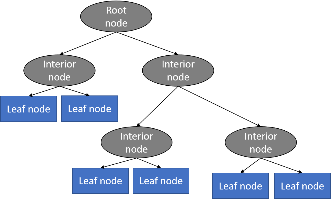
• Each node represents a question about a feature of the data, which can be answered with true or false (branches).

• The process starts at the root node and follows branches based on the answers to these questions, leading to end nodes (also called leaf nodes) that represent the final prediction or class label.

• Easy to understand and visualize.

• Each path from the root to a leaf represents a sequence of decisions leading to a classification.
  
  How it works?

• The tree splits the data by asking questions at each node (e.g., "Is X < -0.25?").

• Depending on the answer, the data follows a branch to the next node, where another question is asked (e.g., "Is Y < -0.75?").

• This continues until a leaf node is reached, which gives the final classification (e.g., "RED" or "BLUE").

SOME TYPES OF ML MODELS USED IN THE AUTOFAB

Support Vector Machine [Slide: 49]

• Supervised ML algorithm used mainly for classification tasks.

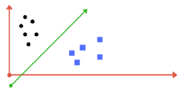
• Works by finding the best boundary (called a hyperplane) that separates data points of different classes.

• Goal: To maximize the margin, (distance b/w the hyperplane and the nearest data points from each class (these points are called support vectors).
  
  How it works:

  • SVM calculates the optimal hyperplane that divides the data into two categories.

  • New data points are classified based on which side of the hyperplane they fall on.

  • The margin should be as wide as possible to improve generalization.

SUPPORT VECTOR MACHINE

Tuning parameters for the hyperplane of SVM [Slide: 50]

1. Regularization Parameter (C)

2. Gamma Parameter

3. Margin
   

1. Regularization Parameter (C)

   • Trades off misclassification of training examples against simplicity of the decision surface.

   • A low C makes the decision surface smooth

   • A high C aims at classifying all training examples correctly.
     

2. Gamma parameter

   • defines how far the influence of a single training example reaches, with low values meaning ‘far’ and high values meaning ‘close’.

   • Gamma can be seen as the inverse of the radius of influence of samples

     selected by the model as support vectors.
     

3. Margin

   • With a high margin, the distance of the training examples to the hyperplane is large on both sides of the line.