Midterm 1 - Units 1-5

Variable

A characteristic that varies; e.g., survey responses like "Yes"/"No".

Dichotomous variable

A variable with exactly two values (e.g., Yes/No).

Categorical variable (Nominal)

Categories without order (e.g., profession, gender).

Ordinal variable

Categories with intrinsic order (e.g., 1=low, 5=high satisfaction).

Numeric variable

Variables with numeric values; can be ordered.

Interval scale

Numeric scale with equal intervals but no true zero (e.g., temperature in °F).

Ratio scale

Numeric scale with equal intervals and a true zero (e.g., weight, income).

Frequency table

Table showing raw counts (frequencies) for each value.

Relative frequency

Proportion of total in each category (e.g., 0.60).

Percentage frequency

Relative frequency expressed as a percent.

Histogram

Graphical display of frequency distributions; bars touch.

Classify each of the following:

• Weight →

• Year of birth →

• Political party →

• Happiness rating (1–5) →

• Religious affiliation (Catholic, Protestant, Muslim, Jewish, etc.) →

• Rating of current happiness on a scale of 1-5 →

• Income in dollars →

• Average monthly temperature →

• Weight →

• Insurance ID number →

• Years of military experience →

• Year of birth →

• Number of answers correct on an exam →

• Political stance, from 1 = Very liberal to 10 = Very conservative →

• Distance between current residence and birthplace →

• Profession/occupation →

• Number of courses taken in the NU School of Professional Studies →

• Weight → Ratio

• Year of birth → Interval

• Political party → Categorical

• Happiness rating (1–5) → Ordinal

• Religious affiliation (Catholic, Protestant, Muslim, Jewish, etc.) → categorical

• Rating of current happiness on a scale of 1-5 → ordinal

• Income in dollars → ratio

• Average monthly temperature → interval

• Weight → ratio

• Insurance ID number → categorical

• Years of military experience → ratio

• Year of birth → interval

• Number of answers correct on an exam → ratio

• Political stance, from 1 = Very liberal to 10 = Very conservative → ordinal

• Distance between current residence and birthplace → ratio

• Profession/occupation → categorical

• Number of courses taken in the NU School of Professional Studies → ratio

Survey responses: Yes (18), No (12)

• Total: ?

• Proportion Yes = ?

• Percentage Yes = ?

Survey responses: Yes (18), No (12)

• Total: 30

• Proportion Yes = 18/30 = 0.6

• Percentage Yes = 60%

Histogram Interpretation (skewed)

If a histogram shows most bars on the left and a long tail on the right → it is positively skewed.

Mean

Arithmetic average

Median

Middle score in ordered data

Mode

Most frequent value

Variance (σ² or s²)

Average of squared differences from the mean; represents how spread out a distribution is, or how dissimilar observations are from each other and from the mean

Standard deviation (σ or s)

Square root of variance (If you know a variable’s variance, you can get its standard deviation simply by taking the variance’s square root. If you know the standard deviation, you can get the variance simply by squaring the standard deviation)

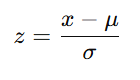
Z-score

Standardized value: how many SDs from the mean

Normal distribution

Symmetrical, bell-shaped curve where most values cluster around the mean

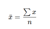
Mean (μ or x̄) equation

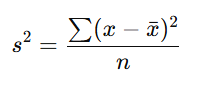
Variance (s²) equation

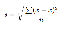
Standard Deviation (s) equation

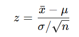
Z-score

Find Mean and SD
Data: [1, 8, 9, 16, 25]

• Mean = 11.8

• Variance = 66.16

• SD = √66.16 ≈ 8.13

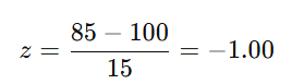
Z-Score Calculation
IQ = 85, Mean = 100, SD = 15

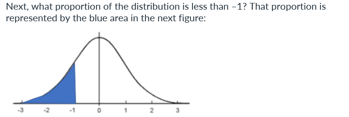
Obviously, this area must be less than half the total, so the proportion is less than 0.5. What do you think it is? Do your best before clicking here to reveal the answer (0.16) = 1/2 - 1/3 = 0.16

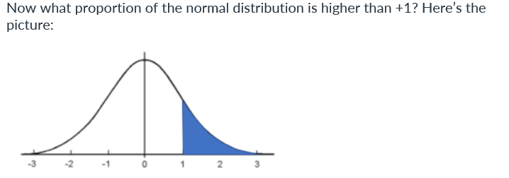
Because the normal distribution is symmetric, the proportion of observations above 1 must equal the proportion below –1, which we already learned is about 0.16. 

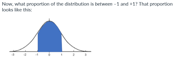
If you estimate this simply by looking at the figure, you will do well if you get near the answer: 0.68. But there is a more straightforward way of getting the answer, using reasoning and the answers we got already: 0.16 of the curve is below –1, and 0.16 is above +1. We want everything else. So the answer is 1 – 0.16 – 0.16 = 0.68

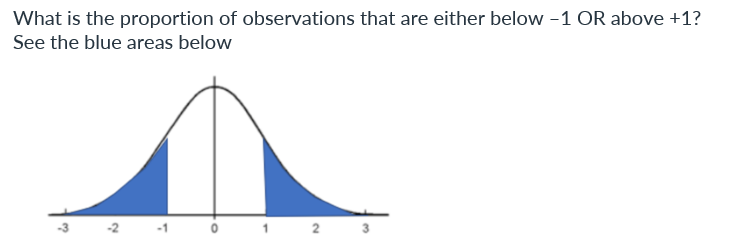
0.16 + 0.16 = 0.33

Check Your Knowledge: Using the Standard Normal Cumulative Probability Table

Use the table to answer these questions. Roll over each question to check your answers.

Provide both the proportions and the percentages of the normal curve that is:

·       Less than –2 standard deviations below the mean? =

·       Greater than –2 standard deviations below the mean? =

·       Greater than 2 standard deviations above the mean? =

·       Either less than –2 standard deviations below the mean or greater than 2 standard deviations above the mean? =

·       Greater than –2 standard deviations below the mean and less than 2 standard deviations above the mean? =

·       Less than –2 standard deviations below the mean? = 0.0228 = 0.023 = 2.3%

·       Greater than –2 standard deviations below the mean? = 1-0.023 = 0.977 = 97.7%

·       Greater than 2 standard deviations above the mean? = 1-0.9772 = 0.0228 = 2.3%

·       Either less than –2 standard deviations below the mean or greater than 2 standard deviations above the mean? = 2 x 0.023 = 0.046 = 4.6%

·       Greater than –2 standard deviations below the mean and less than 2 standard deviations above the mean? = 1-0.046 = 0.954 = 95.4%

standard normal distribution

The standard normal distribution always has a mean of 0 and a standard deviation of 1

Population

Entire group you want to draw conclusions about

Sample

Subset from the population

Parameter

True value in population (e.g., μ, σ)

Statistic

Value from a sample (e.g., x̄, s)

Sampling error

Difference between sample statistic and population parameter

Sampling distribution

Distribution of a statistic (e.g., sample mean) across many samples

Central Limit Theorem

Distribution of sample means approaches normal as sample size increases

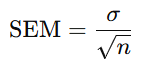
Standard error of the mean (SEM) equation

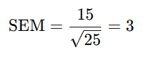
Estimate SEM
Population SD = 15, n = 25

Null hypothesis (H₀)

Assumes no effect or difference (e.g., μ = 100)

Alternative hypothesis (H₁)

Claims an effect or difference (e.g., μ > 100)

Z-test

Compares sample mean to population mean when σ is known

Critical value

Z-score threshold for significance (e.g., ±1.96 for α = 0.05 two-tailed)

Region of rejection

Area in distribution where null is rejected

One-tailed test

Tests for effect in one direction

Two-tailed test

Tests for effect in either direction

Z-test for sample mean equation

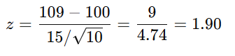
Mozart Babies Example
x̄ = 109, μ = 100, σ = 15, n = 10

p ≈ 0.03 → significant (p < 0.05)

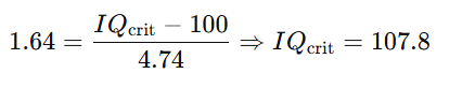
Critical Value
For α = 0.05 one-tailed, critical Z = 1.64
What is the critical IQ value for N = 10?

Sample mean = 106

• Not significant since 106 < 107.8

σ

the population standard deviation for the variable you are analyzing

• If you are using the t-test, then you do not know the value for 

• If you do know , use the Z-test

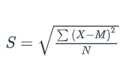
S

refers to the sample standard deviation where M is the sample mean and N is the sample size uses N

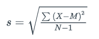
s

refers to the sample estimate of the population’s standard deviation

uses N-1

t versus Z

In the Z-test, we compare a Z score from our sample to critical values of the normal distribution. If we conducted a t-test by hand, we would go through a nearly identical process. You would notice two main differences. First, we would use a slightly different formula to compute our sample standard deviation. (We would use the formula that estimates the population SD from the sample.) Second, we would use a different distribution to compute our critical values. In fact, there is not one t distribution, but a different t distribution for every sample size. 

t distributions associated with smaller samples are wider than those associated with larger samples

For smaller samples, the t distributions are wider (i.e., they have larger SDs).

what is df

degrees of freedom

1.  Other than the Z-test, which does not require degrees of freedom, the statistical tests you will learn are associated with degrees of freedom.

2. I will write “degrees of freedom” and “df” interchangeably.

3. Different statistical tests have different degrees of freedom.

4. For the one-sample t-test, the df are N-1, or one fewer than the sample size.

5. When reporting statistical analyses, you should report df for statistically informed readers, who will want to know. (Otherwise, you can simply tell the less specialized reader your sample size.)

When is a t-test appropriate and a Z-test inappropriate?

If you know the population mean and SD for your variable of interest, you should conduct a Z-test. Otherwise, you must conduct a t-test.

what do exact p-values tell you

whether a result is statistically significant

What is this write up an example of? We examined whether the respondents’ political ideology differed from “moderate,” or a score of 4, as follows: We conducted a one sample t-test using a null hypothesis of 4. The sample mean, 4.05 (SD=1.50) did not differ significantly from 4, t(2246) = 1.55, p = 0.122.

One-Sample t-Test

prob > |t|

two-tailed exact probability - two-tailed exact probability is the probability that if the null hypothesis is true, we will obtain a sample mean more extreme (i.e., farther away from the null hypothesis) than the one we got.

prob > t

one-tailed exact probability for upper tail - the probability that we obtain a sample mean larger than ours

prob < t

one-tailed exact probability for lower tail - the probability that we obtain a sample mean smaller than ours

an ideal candidate for a paired t-test analysis

a pair of variables that are directly comparable because they were answered using exactly the same scale. (In this case, the scale was 1 = very conservative to 7 = very liberal.) And we would like to know about the difference between the two variables.

paired t-test is really doing.

When you can do a paired t-test, and when you can’t

The paired t-test requires that two variables be answered by the same respondents in the same dataset. Furthermore, both variables need to be conceptually and numerically comparable. The example we used was a good one. It makes good sense to compare mothers’ and fathers’ political views, and the variables measuring these used identical scales.