MTH 267 - Differential Equation Final Exam Topics

Reduction of Order

If y₁ and y₂ are linearly independent, then their quotient y₂ ∕ y₁ is nonconstant on I—that is, y₂(x) ∕ y₁(x) = u(x) or ​y₂(x) = u(x)y₁(x).

General Case:

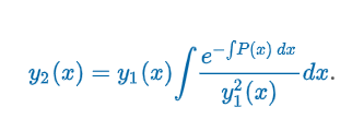
“Let y₁(x) be a solution of the homogeneous differential equation y″ + P(x)y′ + Q(x)y = 0 on an interval I and that y₁(x) ≠ 0 for all x in I. Then (Image) is a second solution.

Note:

Drop the constant!

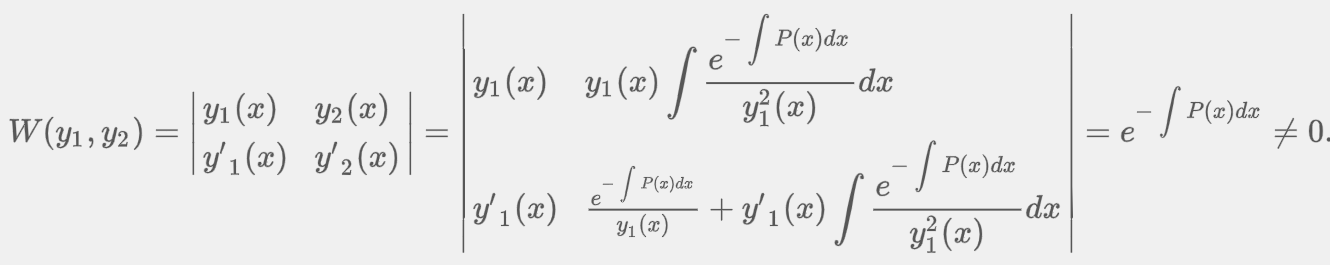
Wronskian w/ Reduction of Order

If is the y₂ solution in the Reduction of Order Formula, then the functions y₁(x) and y₂(x) are linearly independent on any interval I on which is not zero.

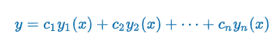
General Solution - Homogeneous

Let y₁, y₂, …, y_n be a fundamental set of solutions of the homogeneous linear -order differential equation on an interval I. Then the general solution of the equation on the interval is y = c₁y₁(x) + c₂y₂(x) + … + c_ny_n(x) where c_i, i = 1, 2, …, n are arbitrary constants.”

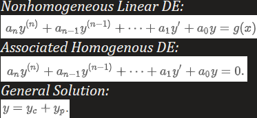
Nonhomogeneous General Solution

General Solution: y = y_c + y_p

y_c : complementary function; general solution of the associated homogeneous DE

y_p :any particular solution of the nonhomogeneous equation

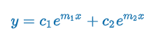
Case 1: Distinct Real Roots (Homogeneous Linear Equations with Constant Coefficients)

Criteria: m₁ & m₂ real & distinct (b² - 4ac > 0)

am² + bm + c = 0 has 2 real unequal roots m₁ & m₂ → linearly independent y₁ = e^m₁x & y₂ = e^m₂x

m₁ = (-b + √(b² - 4ac)) / 2a) & m₂ = (-b + √(b² - 4ac)) / 2a)

y = c₁e^m₁x + c₂e^m₂x

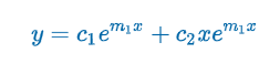
Case 2: Repeated Real Roots (Homogeneous Linear Equations with Constant Coefficients)

Criteria: m₁ & m₂ real & equal (b² - 4ac = 0)

m₁ = m₂ → y₁ = e^m₁x & b² - 4ac = 0 → m₁ = -b/2a

Proof: y₂ = e^m₁x∫(e^2m₁x/e^2m₁x)dx = e^m₁x∫dx = xe^m₁x

m₁ = (-b + √(b² - 4ac)) / 2a) & m₂ = (-b + √(b² - 4ac)) / 2a)

m₁ = m₂ = -b/2a

y = c₁e^m₁x + c₂e^m₁x

Case 3: Conjugate Complex Roots (Homogeneous Linear Equations with Constant Coefficients)

Criteria: m₁ & m₂ conjugate complex numbers (b² - 4ac < 0)

m₁ & m₂ are complex → m₁ = α + iβ & m₂ = α - iβ were α & β > 0 are real & i² = -1

m₁ = (-b + √(b² - 4ac)) / 2a) & m₂ = (-b + √(b² - 4ac)) / 2a)

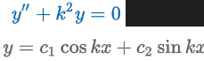
Equation 1 Worth Knowing (Homogeneous Linear Equations with Constant Coefficients)

k: real

DE: y” + k²y = 0

Auxiliary Equation: m² + k² = 0

Roots: m₁ = ki & m₂ = -ki

Solution: y = c₁coskx + c₂sinkx

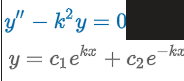
Equation 2 Worth Knowing (Homogeneous Linear Equations with Constant Coefficients)

k: real

DE: y” - k²y = 0

Auxiliary Equation: m² - k² = 0

Roots: m₁ = k & m₂ = -k

Solution: y = c₁e^kx+ c₂e^-kx

Special Case: c₁ = c₂ = ½ → y = 1/2(e^kx + e^-kx) = coshkx

Special Case: c₁ = ½ & c₂ = -½ → y = 1/2(e^kx - e^-kx) = sinhkx

Alternative form: y = c₁coshkx + c₂sinhkx

Rational Roots (Homogeneous Linear Equations with Constant Coefficients)

We know that if m₁ = p ∕ q is a rational root (expressed in lowest terms) of a polynomial equation​ a_nmⁿ + … +a_nm +a₀ = 0 with integer coefficients, then the integer p is a factor of the constant term a₀ and the integer q is a factor of the leading coefficient a_n.​

Method of Undetermined Coefficients

Limited to linear DEs such as nonhomogeneous linear DE where

• the coefficients a_i, i = 0, 1, …, n are constants &

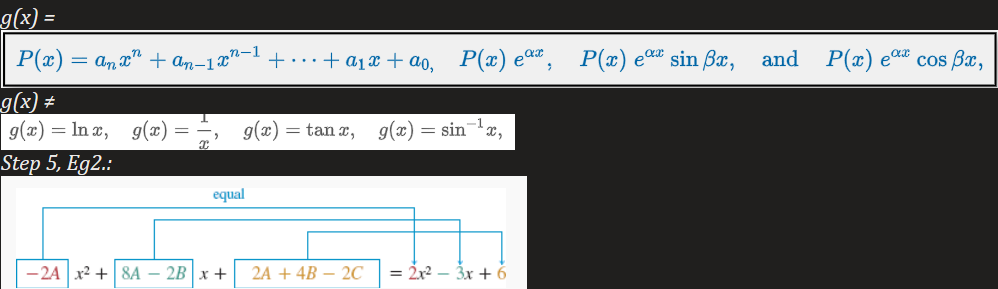
• g(x) is a constant k, a polynomial function, an exponential function e^αx, a sine or cosine function sinβx or cosβx, or finite sums and products of these functions. (Refer to image to what this means)

Steps:

1) Find y_h

• Characteristic Equation

• Identify type of Homogeneous Linear Equations with Constant Coefficient

2) Choose a general y_p

• Look at RHS, the equation will include RHS & it’s derivatives

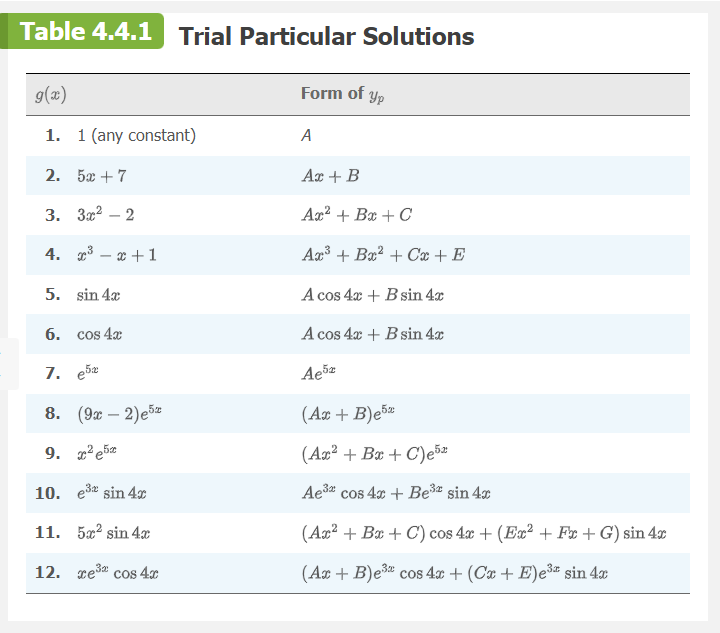
• Refer to Trial Particular Solutions Flashcard

• Eg. RHS = 3x² → Ax² + Bx + C = 0

3) Derive the general y_p

4) Plug the derivatives into the DE

5) Match elements in LHS w/ elements in RHS

• Eg1. LHS = 2A - 4Ax² - 4Bx + 4C; RHS = 3x² + 0x +1 → 2A + 4C = 0, -4B = 0, -4A = 3

• Eg2. Refer to Image

• Solve

6) Plug into y_p

7) Write y = y_h + y_p

8) Check by plugging solution into DE

Superposition Principle for Nonhomogeneous Equations

y_p = y_p1 + y_p2 +…+ y_pn

(Apply this theorem when g(x) is a combination of allowable functions)

Trial Particular Solutions

No function in the assumed particular solution is a solution of the associated homogeneous differential equation.

The form of y_p is a linear combination of all linearly independent functions that are generated by repeated differentiations of g(x).

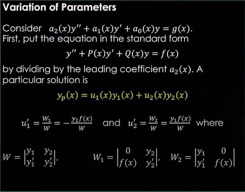
Variation of Parameters

Note: do not need to introduce new constants, solution method may involved integral-defined functions, particular solution may not be unique

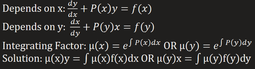
Linear 1st Order DE (Integer Factor)

Follows the linear general formula: a₁(x)(dy/dx) + a₀(x)y = g(x)

Steps:

1) Put into standard form; (dy/dx) + P(x)y = f(x)

2) Identify P(x) & find the integrating factor: μ = e^∫P(x)dx

3) Multiply both sides of the standard form by the integrating factor. The LHS of the resulting equation is the derivative of the product of integrating factor & y.

4) Integrate both sides of the last equation.

5) If asked, solve for y

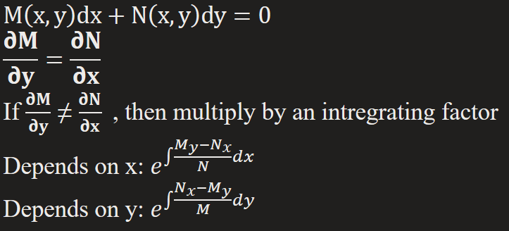
Exact 1^st Order DE

Differential is continuous & has continuous 1^st partial derivatives in R defined by a < x < b & c < y < d on some function f(x,y)

Steps:

1) Set in Exact Equation

• Find the integer factor if necessary

2) Integrate w.r.t. x / Integrate w.r.t. y

3) Partial Differentiate w.r.t. y / Partial Differentiate w.r.t. x

4) Integrate h’(y) / Integrate g’(x)

5) Final answer = C

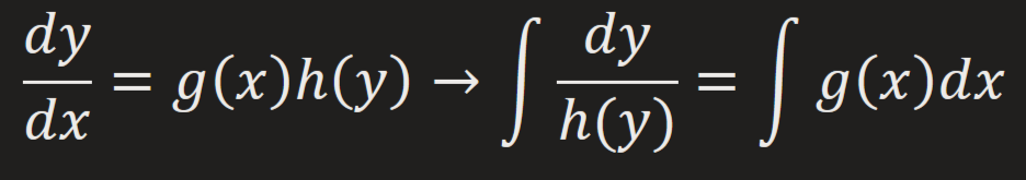
Separable 1^st Order DE

can be separated as a product of a function of x & a function of y (can be linear or nonlinear)

Steps:

1) Separate y terms on the right & x terms on the left

2) Integrate

3) If asked, solve for y

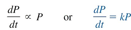
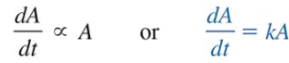
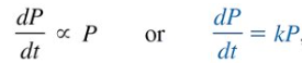
Population Growth

“rate of population growth at a time is proportional to the population at that time”

P(t) = population at time (t)

k = constant of probability

P(t) = P₀(t)e^kt

Note: It is decay if k < 0.

Radioactive Decay

“the rate dA/dt at which the nuclei of a substance decay is proportional to the amount A(t) of the substance remaining at time t”

A(t) = A₀e^-kt

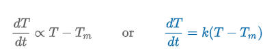
Newton’s Empirical Law of Cooling/Warming

“the rate at which temperature (temp.) of a body changes is proportional to the difference between temp. of body & ambient temp.”

T(t) = T_m + (T₀ -T_m)e^kt

T(t) = temp. of body at time t

T_m = ambient temp.

k = constant of probability

k > 0: warming

k < 0: cooling

Spread of Disease

“the rate dx/dt in which the disease spread is proportional to the number (#) of interactions between diseased people x(t) & unexposed people y(t)”

1^st Order Chemical Reactions

“disintegration of a radioactive substance”

X(t) = amount of substance A at any time t

k = negative constant

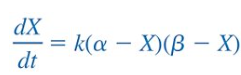
2^nd Order Chemical Reactions

“disintegration of a radioactive substance”

X(t) = amount of C at time t

α = amount of A

β = amount of B

α - X = amount of A not converted to C
β - X = amount of B not converted to C

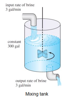
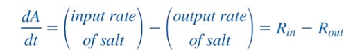
Mixture

“the amount of salt in a mixture of 2 salt solutions of differing concentrations”

A(t) = amount of salt in tank at time t

R_in = input rate of salt

R_out = output rate of salt

R = concentration * rate

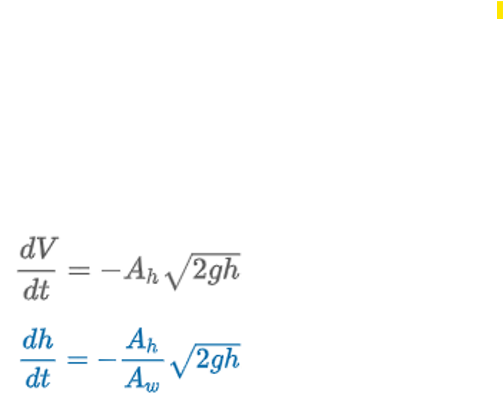
Draining a Tank

“Torricelli’s Law states that the speed of which a fluid flows out of a hole of a container is equal to the speed of it falling freely from the height of the fluid’s surface to the level of the hole.”

A_h = area (ft³) of hole

v = √2gh = speed (ft/s) of water leaving the tank

V(t) = A_wh = volume of water leaving the tank at time t

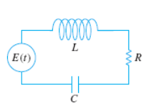
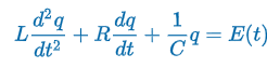
LRC Series Circuit

“Kirchoff’s 2^nd Law states the impressed voltage E(t) in a closed loop equals the sum of the voltage drop.”

E(t) = impressed voltage

i(t) = current in closed circuit

q(t) = charge incapacitor at time t

L = inductance

R = Resistance

C = Capacitance

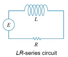
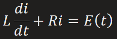
LR Series Circuit

E(t) = impressed voltage

i(t) = current in closed circuit

q(t) = charge incapacitor at time t

L = inductance

R = Resistance

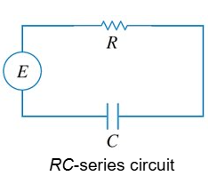
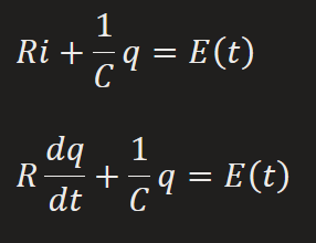
RC Series Circuit

E(t) = impressed voltage

i(t) = dq/dt current in closed circuit

R = Resistance

C = Capacitance

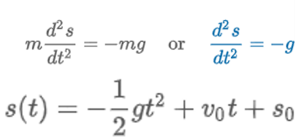
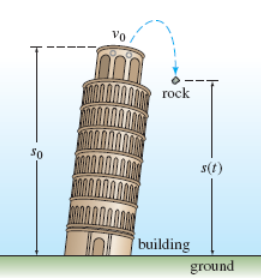
Falling Bodies

“Newton’s 1^st law states a body in motion remains in motion & a body at rest remains at rest unless acted upon by a force. Newton’s 2^nd Law states Force = mass * acceleration.”

s(t) = height position of falling object (obj.)

d²s/dt² = acceleration of falling obj.

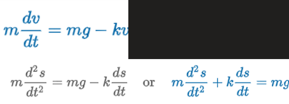
Falling Bodies w/ Air Resistance

“when air is proportional to velocity”

mg = F₁ = W

-kv = F₂ = viscous damping

W = weight

m = mass

g = gravity

s(t) = distance body falls

ds/dt = v = velocity

d²s/dt² = dv/dt = a = acceleration

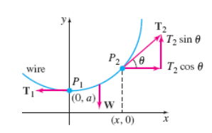
Suspended Cables

“3 forces act on the cables - tension T₁ (tangent to P₁), tension T₂ (tangent to P₂), & Weight W (between P₁ & P₂)

T₁ = cosθ

W = T₂sinθ

tanθ = W/T₁

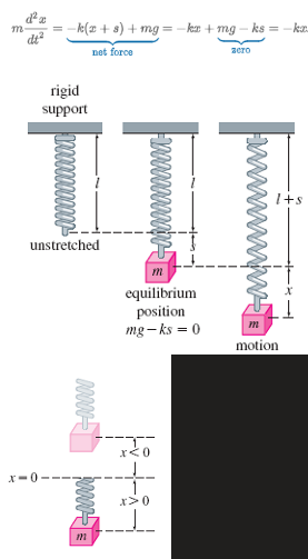
Newton’s 2^nd Law

m(d²x/dt) = -k(x + s) + mg = -kx +mg - ks = -kx

F₁ = -k(x+s) : restoring force

W = mg: Weight = mass*acceleration

• mg = ks or mg -ks = 0: condition of equilibrium (stretched- elongation/compression)

• x(t): displacement where x = 0 is the equilibrium position, above is negative, below is positive

• F = ma: Force = mass* acceleration

• a = d²x/dt²: acceleration

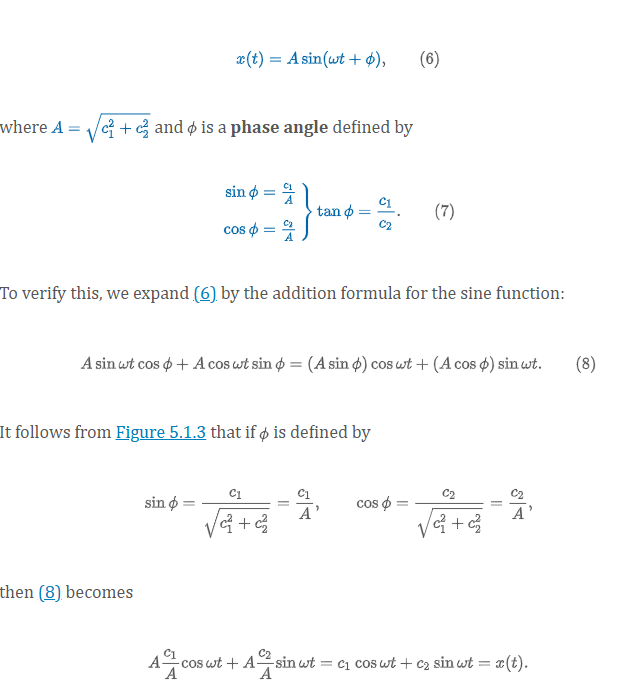
Free Undamped Motion - Alternative Form of x(t)

amplitude A

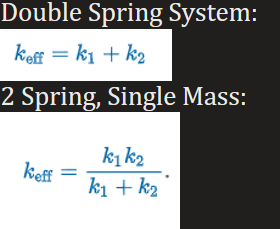
Effective Spring Constant

Spring/Mass Systems: DE of Free Damped Motion

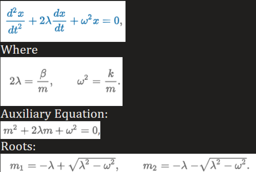
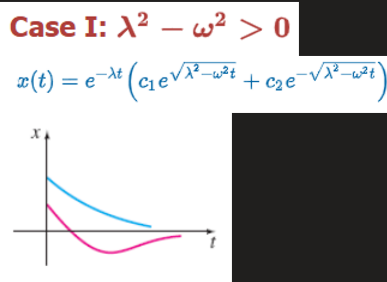
Case 1: Overdamped

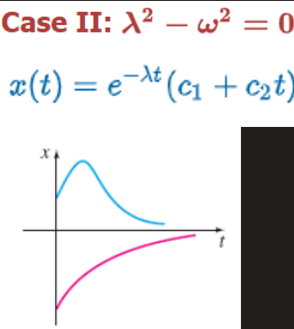
Case 2: Critically Damped

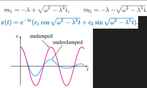
Case 3: Underdamped

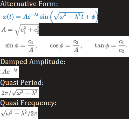
Free Damped Motion - Alternative Form of x(t)

amplitude A

Spring/Mass Systems: Driven Motion with Damping

Take into consideration an external force f(t) acting on a vibrating mass on a spring.

• Note: when F is a periodic function, it is considered a transient term; in other word, y_c = transient term, y_p = steady-state term

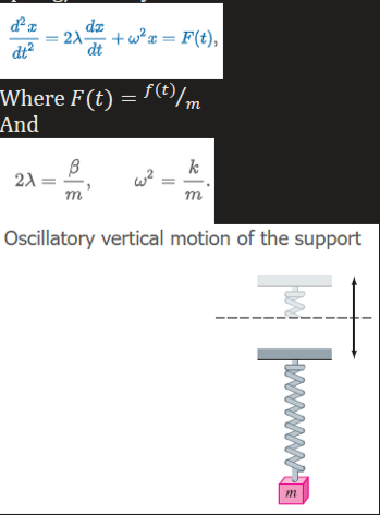
Spring/Mass Systems: Driven Motion without Damping

With a periodic impressed force and no damping force, thereis no transient term in the solution of a problem. ​

LRC Series Circuit

“Kirchoff’s 2^nd Law states the impressed voltage E(t) in a closed loop equals the sum of the voltage drop.”

E(t) = impressed voltage ~ external force, f(t)

i(t) = current in closed circuit

q(t) = charge incapacitor at time t

L = inductance ~ mass, m

R = Resistance ~ damping constant, b

C = Capacitance ~ spring constant, k

• E(t) = 0: electrical vibration of the circuit are free

• E(t) > 0: electrical vibrations are forced

  • R ≠ 0, q_c(t) = transient solution, q_p(t) = steady-state solution

• general solution contains the factor e^-Rt/2L

• the capacitor is charging and discharging as t→∞ (simple harmonic)

• E(t) = 0 & R = 0: undamped, electrical vibrations fo not approach 0 as t increases without bound

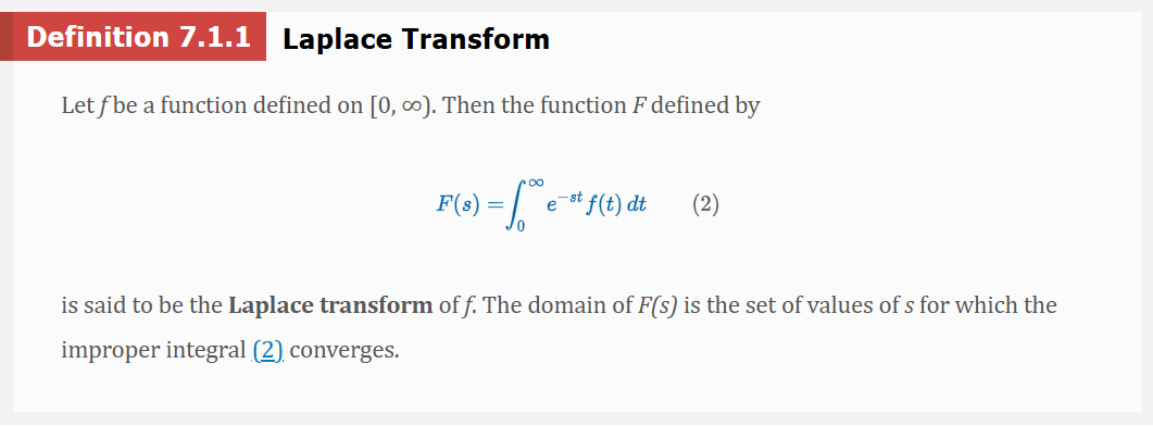
Laplace Transform

Note: also denoted as ℒ{f(t)}

Application: use a lowercase letter to denote the function being transformed and the corresponding capital letter to denote its Laplace transform

ℒ{f(t){ = F(s)

ℒ{g(t){ = G(s)

ℒ{g(i){ = I(s)

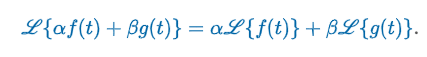
Linear Transform

“Suppose the functions f and g possess Laplace transforms for s > c₁ and s > c₂ , respectively. If c denotes the maximum of the two numbers c₁ and c₂ then for s > c and constants α and β we can write…”

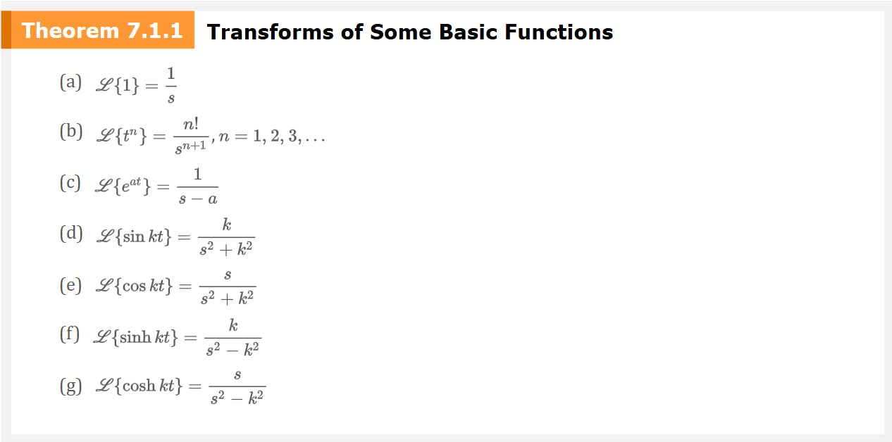
Transform of Basic Functions

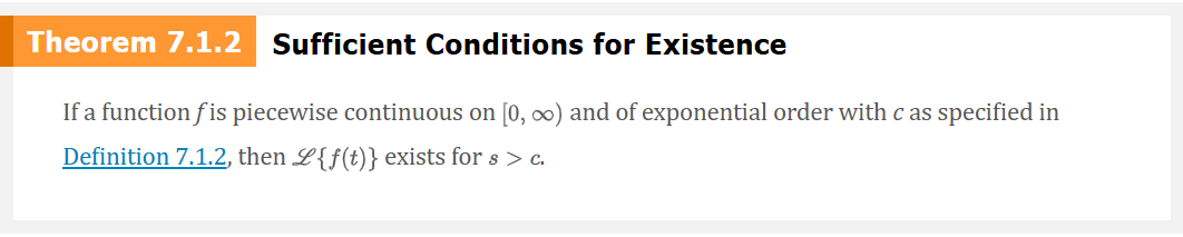
Existence of ℒ{f(t)}

“Sufficient conditions guaranteeing the existence of ℒ{f(t)} are that f be piecewise continuous on [0, ∞) and that f be of exponential order for t > T.”

Inverse Laplace Transforms

Since ℒ{f(t)} = F(s), then f(t)=ℒ^-1{F(s)}

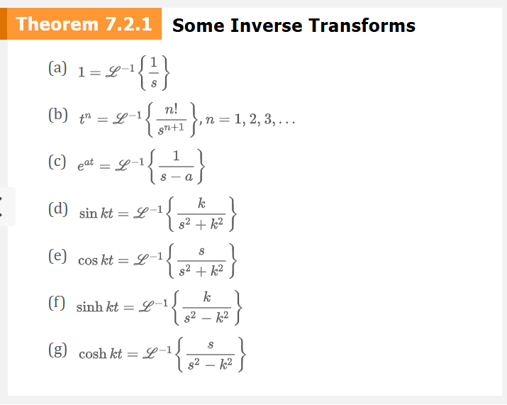
Some Inverse Transforms

Transforms 1^st Derivative

Transforms 2^nd Derivative

Transforms 3^rd Derivative

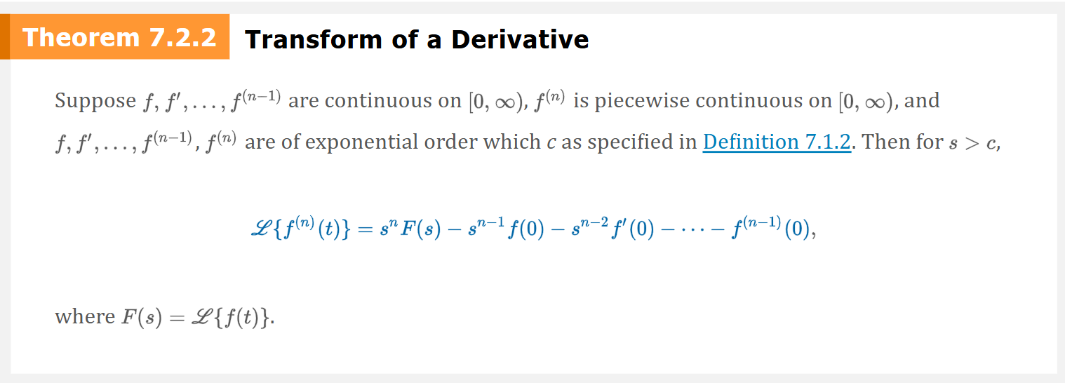
Transform of a Derivative (Theorem)

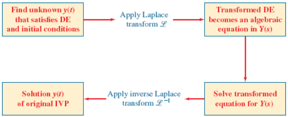
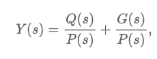
ODE w/ Laplace Transforms

The Laplace transform of a linear differential equation with constant coefficients becomes an algebraic equation in Y(s).

• P(s) = a_nsⁿ + a_n-1s^n-1 + … + a₀

• Q(s) = polynomial in s of degree less than or equal to n - 1 consisting of various products of the coefficient, a₁, i = 1, …, n and the prescribed initial conditions y₀, y₁, …, y_n-1

• G(s) = Laplace transform of g(t)

y(t)=ℒ^-1{Y(s)}

Steps in solving an IVP by the Laplace transform