S1 Aggregate Demand, Fiscal Policy and the National Debt

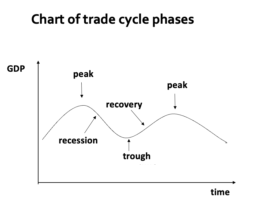
What are cycles in economic activity, what are the phases?

Periodic fluctuations in the rate of economic activity, as measured by levels of employment, prices and production

Peak: the top of the cycle – productive capacity fully utilised shortages may start to develop and the price level may stat to rise faster

Recession: is a downturn in activity. A recession is formally defined as a fall in real GDP for two successive quarters. Typically, incomes and employment levels fall. Profits may also decline as some firms experience financial difficulties. A recession that is deep and long –lasting is called a depression.

Trough: characterised by high unemployment and low demand in relation to the capacity to produce. Business confidence is low

Recovery: characterised by rising incomes, employment and consumption. Business expectations become  more optimistic and new investment projects are begun.

Explain the affect of The Great Depression and the affect on economics.

The Great Depression in the 1920’s had unemployment reaching 2 million in 1922 and peaking at around 3 million (22%) in 1932

This led to the development of Macroeconomics

What did Keynes say about The Great Depression?

‘I know of no British economist of reputation who supports  the proposition that schemes of National Development are incapable of curing unemployment.’

So in his General Theory of Employment, Interest and Money (1936) Keynes argued that effective demand was the key to full employment

Written against the background of the Great Depression the model which underlayed Keynes thinking was based on the short run over which an excess supply of output can prevail, and critically, which would NOT be eliminated automatically (as H.M. Treasury had suggested) .

What are the Income Determination Model Assumptions made by Keynes?

The short run in macroeconomics is different from that in microeconomics: it is traditionally defined as a period over which there is a negative output gap. i.e. the level of demand is less than potential productive potential of the economy (Y<Y*)

Given the short-run nature of the model there are several further simplifying assumptions that Keynes made:

- The industrial structure of the economy is fixed

- Firms’ output is aggregated into a single productive sector producing output which is homogenous

-The price level is fixed: i.e. real and nominal values are identical, or alternatively, all variables are measured in real terms (constant prices)

What was Keynes’s contribution?

Keynes’s most basic contribution was to ask: what determines the level of aggregate expenditure?

Keynes divided total production into consumption goods (C) – purchased by households and capital goods (investment, I) – purchased by firms.

If he could explain the determinants of C and I he would have a theory of aggregate spending.

In terms of a model of C and I Keynes divided each into autonomous and induced spending

  -  Autonomous (or exogenous) spending is that spending which is independent of    current income

  -  Spending which rises with income is referred to as induced spending

Explain the MPC and the APC

‘The fundamental psychological law, […] is that men are disposed, as a rule and on the average, to increase their consumption as their income increases, but not by as much as the increase in their income.’ - Keynes

The fundamental psychological law implies a new concept: the marginal propensity to consume (MPC).

This is defined as: ΔC/ ΔY where  0 < ΔC/ ΔY < 1. This says that the change in consumption is less than the change in income

Keynes also argues that the MPC is smaller at higher levels of income and larger at lower levels of income (so the implied consumption function is non-linear)

Keynes also says that “on average” C and Y will rise (or fall) together. This is called the average propensity to consume (APC) - defined as: C/Y

Keynes believed that the C/Y ratio would fall as incomes increased: “…a greater proportion of income being saved as real income rises.” [GT p.97] (This also implies that the consumption function is not linear.)

Explain the formal linear relations for this

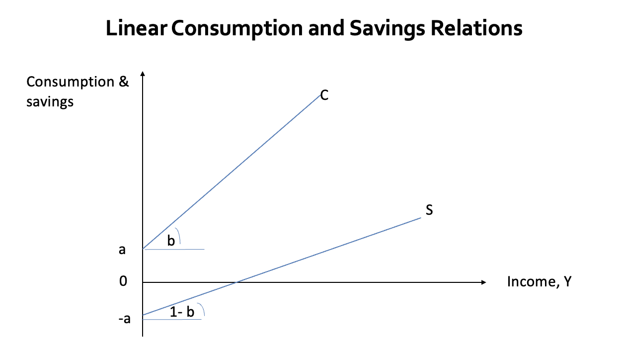
For simplicity we assume that consumption can be represented by a linear equation:

     C = a + bY  

  where: a is autonomous consumption

        b is ΔC/ΔY = the marginal propensity to consume (mpc)

Note also the average propensity to consume (apc) falls as income rises as C/Y = (a/Y) +b (autonomous consumption takes up a lower proportion of Y)

Since income is either consumed or saved then Y = C + S and saving, S can be written as:

  S = Y – C = – a +(1 – b)Y

Thus savings are also a positive function of income, with a marginal propensity to save (MPS) of (1 – b) and a negative intercept of – a. 

Note also the APS rises with income as S/Y = -(a/Y)+(1 - b)

What is the role of investment in Keynesian economics, and how does it relate to the aggregate expenditure function in an economy without government or trade?

Investment: The most volatile component of GDP and the hardest to forecast. Keynes believed it is driven by business expectations.

Investment is assumed to be exogenous (independent of income).

In an economy without government or trade, the aggregate expenditure (AE) function is: AE = C+I

According to Keynes, AE determines the level of output (Y): AE = C + I = Y 

Combining the two parts of AE: AE = a + bY + I

At equilibrium (AE=YAE = YAE=Y):

• Intercept = a + I

• Slope = b (marginal propensity to consume).

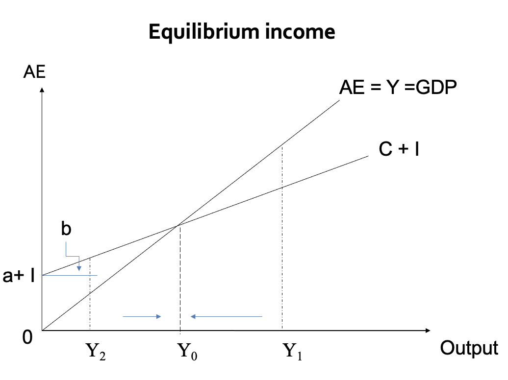
Explain the Equilibrium income graph

The AE = Y line is the set of equilibrium points between expenditure and income

The C+I line is the planned (or desired) total expenditure function (AE)

At Y₀ planned expenditure is exactly equal to income so Y is constant

At Y₁ planned spending is less than output so income will fall back to Y₀ due to lack of demand

At Y₂ planned spending exceeds output so firms expend production to Y₀ to meet the excess demand

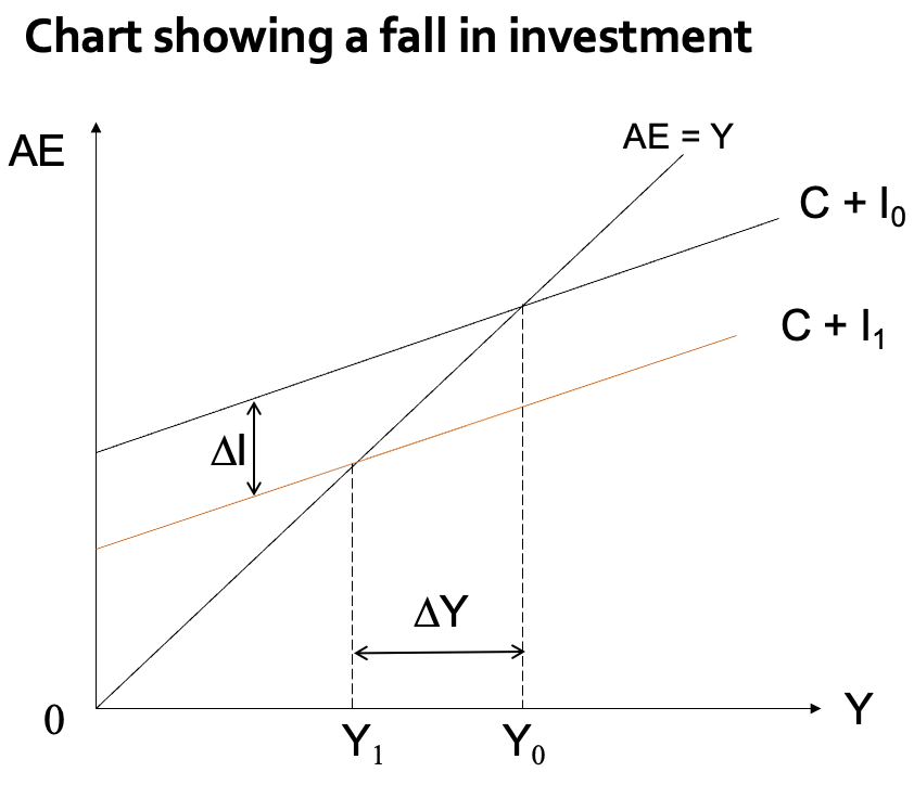
What effect does a fall in autonomous investment have on this graph?

To be able to use the model it needs to be disturbed from its equilibrium by an exogenous shock.

Suppose from the initial level of equilibrium income there is a fall in investment from I₀ to I₁ , where I₀ > I₁

The level of AE will fall and the level of equilibrium output will fall from Y₀ to Y₁

There are 2 things to note about the diagram:

- The fall in I is a parallel downward shift in the C+I line

- The fall in Y is greater than in the fall in I. (To see this compare the vertical distance ∆I with the horizontal distance ∆Y)

This is called the multiplier effect – where the fall in investment has a magnified effect on output.

The size of the multiplier (k) is given as: k = 1/(1-b) =  1/mps  = 1/(1-mpc)

Explain the Multiplier, and its relation to the previous graph.

The multiplier refers to the process by which an initial change in spending (such as investment, government spending, or consumption) leads to a larger overall change in output (GDP) or income in the economy.

To see how this result is obtained recall the formal 2-equation model:

    C = a + bY  and  AE = Y = C + I

Substituting for C into AE gives: Y = a + bY + I    so    Y(1 - b) = a + I.

Then dividing both sides by (1 – b)  gives: Y= (a + I)/(1 - b) = k (a + I) so k =  1/(1-b)

So any change in I, say ΔI, leads to a change in income (ΔY) of k ΔI; i.e. ΔY/ΔI = k.

Suppose that b = 0.75. Then the multiplier (k) is 1/(1 – b) = 1/0.25 = 4. So any change in I has an effect on Y which is 4 times larger than the change in I.

There is a direct relationship between the size of the mpc (i.e. b) and the size of k.

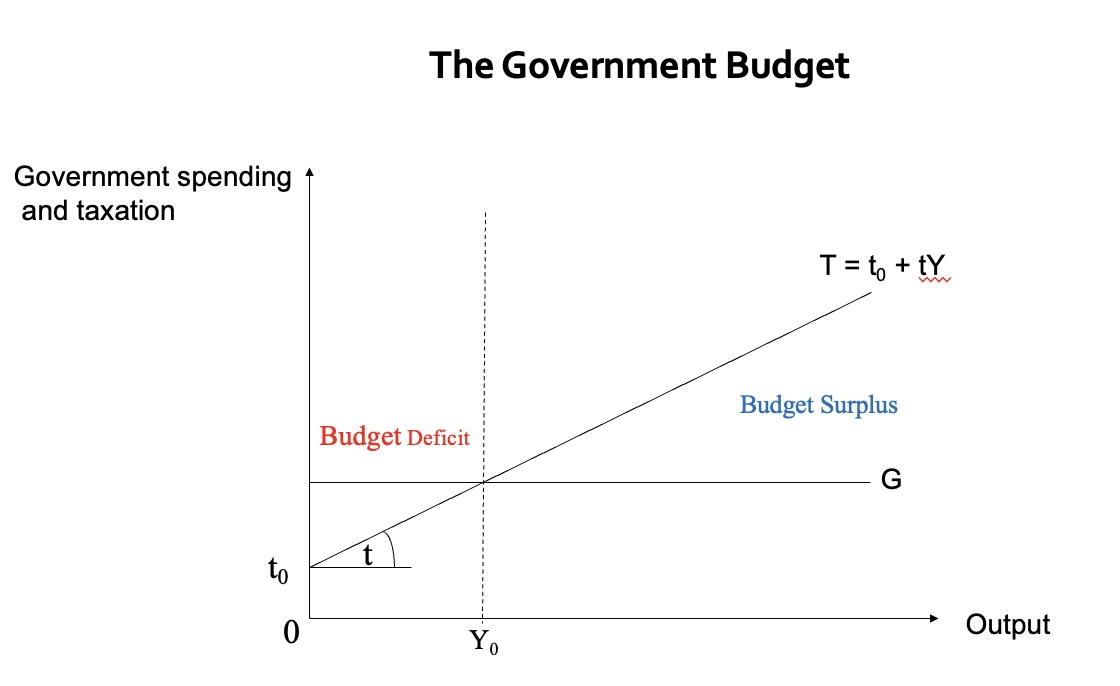
Explain the Government Sector

The government sector consists of exogenous government spending (G) and endogenous (net) tax revenues (T).

G is assumed to be exogenously given by the need to fund public services such as defence the police.

Net tax revenues are defined as tax revenues less transfer payments made. Since tax revenues always exceed transfer payments, net taxes are always positive. We write the tax (or net tax) function as:

  T = t₀ + tY

t is the marginal propensity to tax (MPT) and t = ΔT/ΔY,

t₀ denotes autonomous taxes – not related to income, such as VAT.

Note that some of T is endogenous, which makes the government budget, T – G, endogenous and beyond the control of government itself.

Explain the Extended Formal Model

With government the income identity is now: AE = Y = C +I + G

Consumption is now a function of disposable (post-tax) income so: C = a + b(Y - T)

Tax revenue is: T = t₀ + tY

Substituting gives equilibrium income as:  Y = (a - bt₀+I+G)/(1-b(1-t))

Notice now the multiplier has a different value: k_G = 1/(1-b(1-t)). Since t >0 the multiplier must be smaller than before when t = 0

Note also the additional elements in autonomous expenditure; government spending, G and autonomous taxes, t_0. These are the parameters of discretionary fiscal policy.

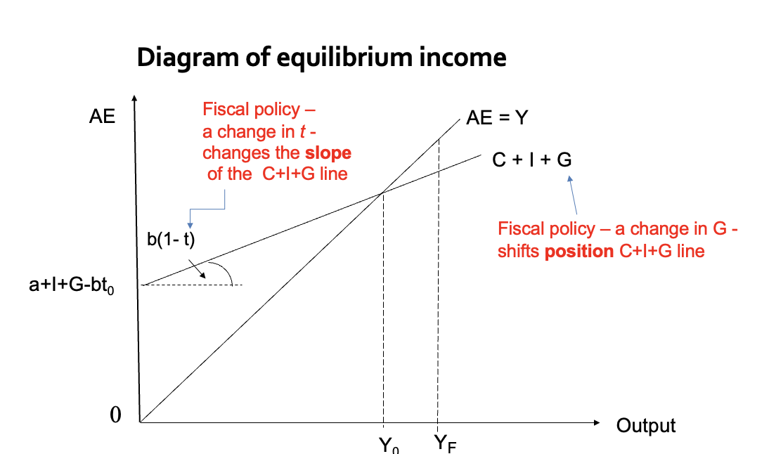
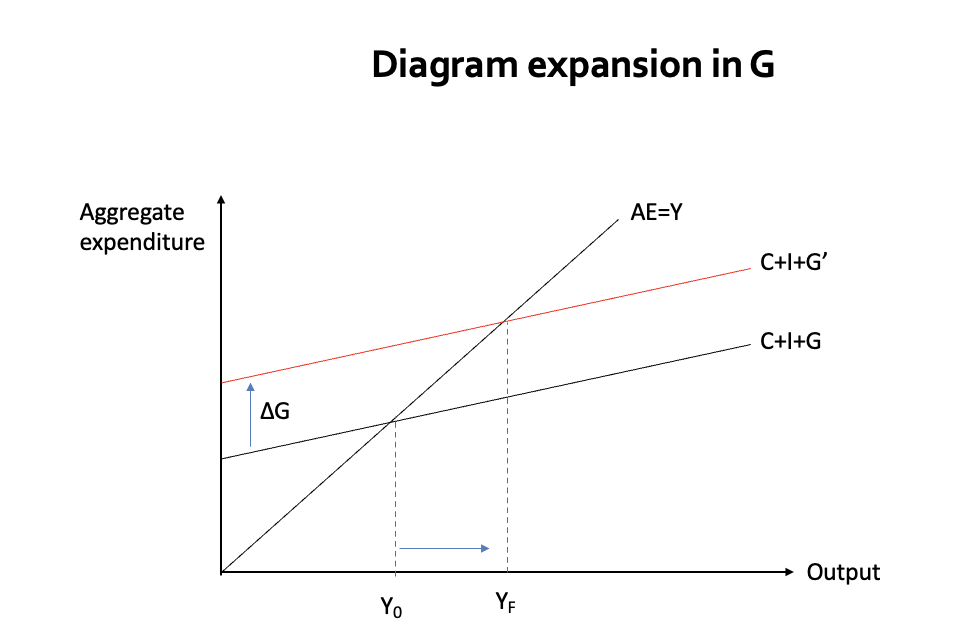
Explain how fiscal policy affects the graph

Suppose the full employment level of income is at Y_F, then by changing G, t₀ or t governments can affect the level of AE and hence raise output from Y₀ to Y_F.

Such discretionary fiscal policy changes have different sized multiplier effects:

 - changes in G and t₀ will cause the AE-line to shift, but the increase in G necessary to move the model to Y_F will be more certain and less than the cut in t₀.

 -  changes in t will cause the line to swivel; e.g. a lower value of t, causes the AE line to swivel anti-clockwise

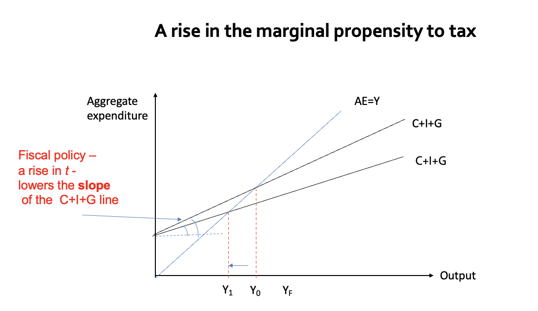
How does a change in the tax rate affect the graph?

The maths are slightly more complicated in this case. The model is, as before:

  Y= a + b(Y – t₀ – tY)+ I+ G

Taking changes of Y and t gives:  ΔY = a + b(ΔY – t₀ – t ΔY – Y Δt) + I + G

Grouping terms together` gives: ΔY(1 – b(1 – t))= – b Y Δt + a bt₀ + I+ G

Finally, re-arranging and ignoring the constant the new marginal tax rate multiplier is    "ΔY" /"Δt"   = "– b Y" /"1 – b(1 – t) "  = k_t  

This multiplier is negative because a rise in the tax rate reduces income, but by how much depends on the initial level of income. The following chart shows this.

What is the difference between automatic and discretionary fiscal policy?

Automatic Stabilizers:

Policies that automatically adjust without new government action, such as:

Unemployment benefits (increase when unemployment rises).

Progressive taxes (tax revenue falls when incomes decline).

Discretionary Fiscal Policy:

Deliberate changes in government spending or taxation decided by policymakers.

The government’s budget can be written as: (G –T ) = G – (t₀ + tY).

So any rise in Y increases tax revenue without any change in t (or G). So in a boom period the government deficit will automatically fall and in slump periods it will automatically increase without any discretionary  change in policy.

Explain the HEBS (Household Economic Behaviour Surveys)

To allow for the fact that part of the budget is endogenous - indeed G may also rise endogenously as GDP falls (extra benefit payments, for example) - to measure a government’s fiscal stance we need to measure it at the “full employment” or “capacity” level of income.

The main problem with this measure is that the potential level output is not known and has to be estimated first.

Then the fiscal policy stance (FPS) can be measured as:  FPS = (G – T)/Y*, where Y* is the full capacity level of income. 

In practice, however, it is often just measured as the simple ratio  (G –T )/Y, which is not immune from all cyclical fluctuations, but at near full employment levels of output is deemed to be good enough to set targets for.

What are the timing problems with Discretionary policy?

Although a good solution to a depression, or prolonged recession, discretionary fiscal policy is more difficult to implement in normal periods. If actions are mis-timed they can lead to exacerbating the cycles rather than damping it.

There are 4 main time lags which are problematic:

Recognition/Identification lag – time taken to realise that there is a problem. Often due to data collection.  

Response lag – time taken to analyse the data and propose a policy change

Execution lag – time taken to get approval from cabinet/parliament and to   implement policy change

Outside lag – time taken for policy changes to work through the economy  to affect target variables.

What are Fiscal rules?

Fiscal rules have been in fashion since the early 1990s although they have been notably unsuccessful in constraining  deficits or debt levels

The Maastricht Treaty (1992) proposed two (political) rules:

  (i) (G-T)/GDP < 3%  and   (ii) Debt/GDP < 60%.

These rules were broken immediately by the major EU economies, France, Italy, Belgium, Greece etc. and have been wholly ineffective even within a monetary union.

The UK did not breach either of these rules and the fiscal rules in the UK since 1997, distinguished between capital spending and current spending. Tax revenues to fully cover current spending; and borrowing only permitted for investment spending.

The Debt/GDP rule is about sustainability and is perhaps the more important because it gives a measure of the accumulation of national debt

What is the Rule of Thumb for debt to GDP ratio?

As a rule the debt to GDP ratio will fall if the real rate of interest (r – π) is less than the growth rate, Ɣ; i.e. if  r – π < Ɣ   or    r < Ɣ+ π.

This is the real concern with the recent budget. With growth predicted to be only about 1-1.5 % over the Parliament, inflation targeted at 2%, then for the debt /GDP ratio to be falling then nominal interest rates must not exceed 3- 3.5%. This seems unlikely – probably meaning further tax rises in the future budgets.

If inflation is allowed to exceed the target of 2% - say to 4% or 5 % - then even with low growth r need not exceed 5% or 6%.

Confirming the inflation target of 2% the chancellor has ruled out the way other high debt burden – say since 1945  - have been reduced by creeping inflation!

What are imports and exports?

Exports are goods and services made in the UK but sold abroad. As the drivers of exports - foreign income and foreign price competitiveness are largely exogenous -  we assume that exports, X, are exogenous.

Imports, M, are goods and services made abroad but purchased by UK residents

Imports rise with domestic income and rise with the price competitiveness of foreign goods; i.e. as home prices rise relative to foreign prices the demand for imports rises.

Since price competitiveness is largely exogenous, imports can be written as a linear function:

  M = m₀ + mY,   where 0 < m < 1

  where m is the marginal propensity to import (MPM),

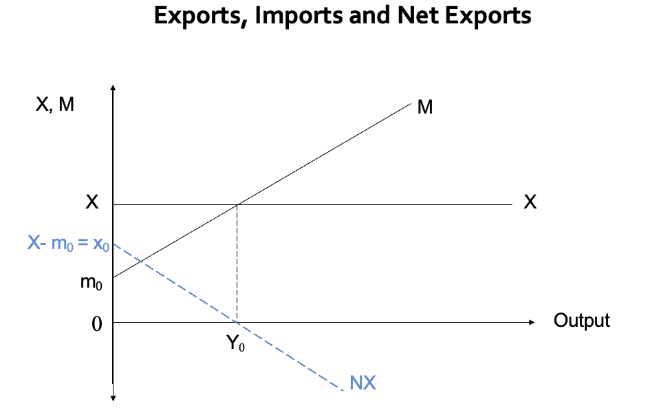
What are net exports?

Net exports (NX) are exports less imports:

NX = X - M  or  NX = (X – m₀) – mY  =  x₀ – mY ,   where (X – m₀) = x₀

An exogenous rise in foreign GDP causes the demand for exports to rise. This causes NX to shift upwards, as X and x₀ rise. Similarly, a fall in foreign GDP causes NX to shift downwards

AE = C + I + G + X – M  = C + I + G + NX 

What is the full model of Income Determination now?

The full model of equilibrium GDP is now:

  AE = Y = C + I + G + NX

       = a + b(Y –t₀ – tY) + I + G + x₀ – mY

 which gives in equilibrium, when AE = Y

  Y = (a – bt₀ + x₀ + I + G)/ [1– b(1 – t) + m]

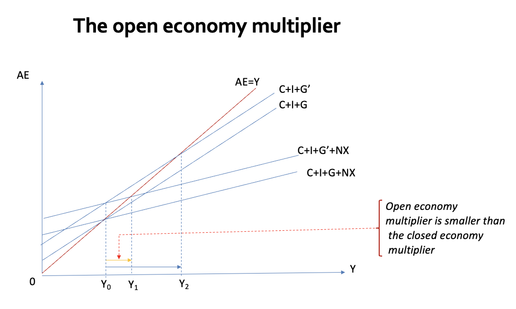
Thus the open economy multiplier with government (k_o) is:

  k_o = 1/ [1– b(1 – t) + m]

This is smaller than the previous multipliers because m>0; so we have that:  k > k_G > k_O

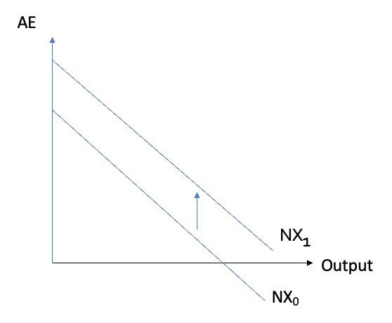
What may shift the NX line?

Foreign incomes and relative international prices.

A rise in foreign incomes will lead to a rise in exports, causing the X-line to shift up (and the NX line) to shift up.

Any change in the relative prices of home-produced goods relative to those of foreign goods will cause both imports and exports to change:

• a rise in domestic prices relative to foreign prices: foreigners will see domestic goods as more expensive and home exports will fall. Domestic residents, on the other hand, will find foreign goods relatively cheaper and imports will increase and the NX schedule will shift downwards

• if home and foreign prices are constant but the exchange rate of sterling depreciates – this makes imports more expensive and exports cheaper and the NX schedule will shift upwards

What are the components of the relative international price ratio (competitiveness) and how does it relate to the real exchange rate?

The relative international price ratio (competitiveness) has three components:

1. Domestic price level, P

2. Foreign price level, P*

3. Exchange rate, E

   Competitiveness (q) is written as: q = PE / P*

   Here, E is the foreign (dollar) price of a pound. For example, E = $1.30 means 1 pound = 1.30 US dollars.

   If prices are constant (P = P* = 1), then q = E.

   A depreciation of E leads to a fall in q (an improvement in UK competitiveness).

   • This depreciation increases exports, reduces imports, and shifts the NX schedule upwards.

   • A fall in E can raise Aggregate Expenditure (AE) in an open economy.

Why does the NX line shift up?

• exports rise (say due to a rise in foreign incomes)

• a depreciation of the pound, which makes exports cheaper and imports more expensive so leading to a switching of expenditure to domestic production and away from foreign  output.

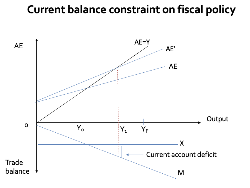
Why is fiscal policy less effective in an open economy, and how does the trade balance impact expansionary fiscal policies?

In an open economy, fiscal policy effectiveness is reduced because higher income from fiscal expansion increases imports (lower net exports), which act as a withdrawal from the circular flow of income.

The trade balance deficit (net exports) can act as a constraint on expansionary fiscal policies, particularly under a fixed exchange rate policy.

• While deficits can be financed by borrowing from abroad in the short run, this is unsustainable. Eventually:

  1. The country may be forced to devalue its currency, or

  2. Reverse the fiscal expansion.

• A diagram can show the impact of a tax cut on GDP and the trade balance by plotting net exports (NX) below the AE line.

What constraint does the current account impose on fiscal expansion under a fixed exchange rate, and how does the Swan Model address it?

The current account of the balance of payments is a constraint on fiscal expansion under a fixed exchange rate.

• In an open economy, there are two policy objectives:

  1. Internal balance (full employment)

  2. External balance (current account balance)

• The problem: Only one policy instrument (fiscal policy) is available.

• Tinbergen’s Rule states: To achieve two targets, you need two policy instruments.

• Solution: Use the nominal exchange rate (E) as the second instrument.

  • With two instruments (fiscal policy and exchange rate), both objectives can be achieved simultaneously.

• This concept is known as the Swan Model of open economy economic policy.

Explain the Swan Diagram

In Zone I:  NX>0, AE>Y

In zone II: NX<0, AE>Y

In zone III: NX<0, AE<Y

In zone IV: NX>0, AE<Y

A vertical disequilibrium along the dotted line can be corrected by changing q alone

A horizontal disequilibrium along the dotted line can be corrected by changing G alone

A diagonal disequilibrium requires the adjustment of both instruments

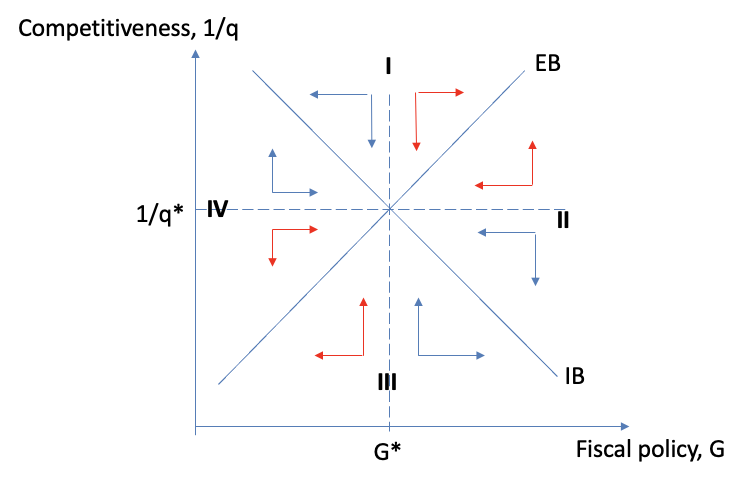
What does the diagram show?

This model shows that to reach the bliss point requires two policy instruments used in an appropriate combination

In every case knowledge about the position of the economy is crucial to understanding the policy combination required. Since in every zone one policy instrument is ambiguous – you need to know where in the zone you are! In practice excellent forecasting is important, but probably also unachievable

It is a static diagram - and as policies take time to have their full effect as they work through the system – so some key variables may move in the wrong direction to begin with

This shows how difficult demand management is likely to be in the real world even with adjustable exchange rates. The diagram can also be used to show why monetary unions (or fixed exchange rate regimes)  often fail.