CPSC 428: Applied Machine Learning

Supervised Learning

• Uses known features to predict an unknown output

  feature (requires training)

• Requires labeled data

  • Training: Learn from examples -> generalize model

  • Bad data -> bad models

• 2 Types: Regression and Classification

What are some steps in sentiment analysis?

tokenization, removing stop words, stemming

When creating a sentiment analysis model to examine words or sentences, what should your first layer of your model be?

Embedding

 What is the purpose of padding a sequence when performing sentiment analysis?

To equalize the sequence

What are the six different types of bias large language models are vulnerable to?

Algorithm, Sample, Anchoring, Availability, Confirmation, Exclusion

What are the three layers of neural networks?

Input layer, hidden layer, output layer

What do transformers allow computer to do?

Allows us to process input concurrently instead of sequentially

Feature transformation

involves manipulating the features or variables in a dataset to improve the performance of a machine learning model or to better understand the relationships between variables. Feature transformation is often combined with other techniques such as data collection, model training, and model evaluation to create effective and accurate models for a wide range of applications.

Single-value imputation

is a univariate imputation technique that involves replacing missing values with a constant such as the mean, median, or mode. Although easy to implement and computationally inexpensive, single-value imputation has the following limitations and potential problems:

• Distortion of data — The feature's distribution will be weighted heavily toward the single-value estimate after imputation.

• Underestimation of variance and standard errors — Statistical methods that are sensitive to variance and standard errors such as hypothesis testing and confidence intervals will lead to inaccurate results.

Univariate imputation

algorithms replace values for a feature using only non-missing values for that same feature.

Multivariate imputation

use regression models to predict the missing values based on the other features in the data. Multivariate imputation can handle both linear and nonlinear relationships between the features but assumes that the data is normally distributed and the missing values do not affect the regression model. The output feature(s) should not be used for multivariate imputation to avoid bias during model training.

k-nearest neighbors imputation

uses the k most similar instances to a data point to impute the missing values. This technique can handle both numerical and categorical data. knn imputation preserves the distribution of data and is more robust to outliers compared to single-value imputation techniques that use the mean or median. Since knn is a distance-based algorithm, normalization or standardization is required, especially when the features have different units.

Steps for Linear Regression

1. read in data

   diamonds = pd.read_csv('diamonds.csv')

2. define features

   X = diamonds[['carat', 'table']]
   y = diamonds['price']

3. Initalize Model

   multRegModel = LinearRegression()

4. Fit Model

   multRegModel.fit(X,y)

5. Get intercept

   intercept = multRegModel.intercept_

6. Get coefficients

   coefficients = multRegModel.coef_

7. Predict

   prediction = multRegModel.predict([[5, 2]])

Steps for Elastic Net Regression

1. read in data

   diamonds = pd.read_csv('diamonds.csv')

2. define features

   # Define input and output features
   X = diamonds[['carat', 'table']]
   y = diamonds[['price']]

3. Scale the features

   # Scale the input features
   scaler = StandardScaler()
   X = scaler.fit_transform(X)

4. Initialize Model

   
   # Initialize a model using elastic net regression with a regularization strength of 6, and l1_ratio=0.4
   eNet = ElasticNet(alpha=6, l1_ratio=0.4)

5. Fit Model

   # Fit the elastic net model to the input and output features
   eNet.fit(X,y)

6. Get intercept

   # Get estimated intercept weight
   intercept = eNet.intercept_
   print('Intercept is', np.round(intercept, 3))

7. Get coefficients

   # Get estimated weights for carat and table features
   coefficients = eNet.coef_
   print('Weights for carat and table features are', np.round(coefficients, 3))
   

8. Predict

   prediction = eNet.predict([[carat, table]])
   print('Predicted price is', np.round(prediction, 2))

Steps for KNN Regression

1. read in data

   diamonds = pd.read_csv('diamonds.csv')

2. define features

   # Define input and output features
   X = diamonds[['carat', 'table']]
   y = diamonds['price']

3. Initialize Model

   # Initialize a k-nearest neighbors regression model using a Euclidean distance and k=12 
   knnr = KNeighborsRegressor(n_neighbors=12, metric="euclidean")

4. Fit Model

   # Fit the kNN regression model to the input and output features
   knnrFit = knnr.fit(X,y)

5. Predict

   # Create array with new carat and table values
   Xnew = [[carat, table]]
   
   # Predict the price of a diamond with the user-input carat and table values
   prediction = knnrFit.predict([[carat, table]])
   print('Predicted price is', np.round(prediction, 2))

6. get nearest neighbors distance

   # Find the distances and indices of the 12 nearest neighbors for the new instance
   neighbors = knnrFit.kneighbors(Xnew)
   print('Distances and indices of the 12 nearest neighbors are', neighbors)

Steps for KNN Classifier

1. read in data

   # Load the dataset
   skySurvey = pd.read_csv('SDSS.csv')

2. define features

   # Create a new feature from u - g
   skySurvey['u_g'] = skySurvey['u'] - skySurvey['g']
   
   # Create dataframe X with features redshift and u_g
   X = skySurvey[['u_g','redshift']]
   
   # Create dataframe y with feature class
   y = skySurvey[['class']]

3. Split data is applicable

   X_train, X_test, y_train, y_test = train_test_split(X, y, test_size=0.

4. Initialize Model

   # Initialize model with k=3
   skySurveyKnn = KNeighborsClassifier(n_neighbors=3)

5. Fit Model

   # Fit model using X_train and y_train
   skySurveyKnn.fit(X_train, np.ravel(y_train))

6. Predict

   # Find the predicted classes for X_test
   y_pred = skySurveyKnn.predict(X_test)

7. get score

   # Calculate accuracy score
   score = skySurveyKnn.score(X_test,np.ravel(y_test))

Hyperparameter

user-defined setting in a machine learning model that is not estimated during model fitting. Changing the values of a hyperparameter affects the model's performance and predictions.

an example would be k in knn

Unsupervised Learning

• No labeled data, good for data exploration &

  finding hidden patterns, automatic processing

  (no training), no prediction

• 3 Types: Clustering, Association, and Dimensionality Reduction

Euclidean Distance Formula

d = √[(x₂ – x₁)² + (y₂ – y₁)²]

Manhattan Distance Formula

The Manhattan distance formula, also known as the L1 distance or taxicab distance, calculates the distance between two points in a grid-like space by summing the absolute differences of their coordinates: |x1 - x2| + |y1 - y2|

Minkowski Distance Formula

The Minkowski distance formula, a generalized way to measure distance between two points in a vector space, is (∑ |uᵢ - vᵢ|ᵖ)¹/ᵖ, where 'p' is a parameter that determines the type of distance (e.g., p=1 for Manhattan, p=2 for Euclidean). 

Dimensionality Reduction

• Reduce the number of features (=>faster processing)

• Sometimes part of pre-processing data (e.g., for

supervised learning)

Reinforcement Learning

• Feedback based algorithms where future

  decisions are made on previous outcomes.

• “Good” decisions get rewards, “bad” ones don’t.

• Algorithm evolves over time.

• Examples:

  • Self-driving cars/robotics

  • Stock Market

  • Playing games

Features

• input into the model

• X

Labels

• correct outputs

• y

Clustering

unsupervised learning task in which instances are grouped based on similarities in the input features. Since clustering is unsupervised, no target output features exist. Instead, clustering results in a new feature containing group assignments. Clustering algorithms use similarity measures to group instances, such as distance or correlation. Applications of clustering include customer segmentation, recommendation systems, and social network analysis.

Classification

• Based on labeled training data identifying

  membership of individual items in distinct groups,

  the algorithm will predict membership, i.e.,

  classify, unseen data into one of the groups.

• Requires a training and testing phase

• Common classification algorithms are

  • KNN

  • Logistic Regression

  • Decision Trees & Forests

Steps of Machine Leaning

Testing Set

used to fit the initial model.

Training Set

used to evaluate a model's performance or select between competing models.

Validation Set

used to decide optimal hyperparameter values or assess whether a model is overfitted or underfitted.

Underfitting

the model is too simple to fit the data well. Underfitted models do not explain changes in the output feature sufficiently, and will score poorly during model evaluation.

Overfitting

the model is too complicated and fits the data too closely. Overfitted models do not generalize well to new data. A model that fits the general trend in the data without too much complexity is preferred.

Varience

• model's sensitivity to fluctuations in the training data, leading to overfitting when high, where the model captures noise and performs poorly on unseen data

• Variance is a measure of how much a model's predictions vary when trained on different subsets of the training data.

• Low variance → less sensitive to change

• high variance → sensitive to change; fits training data too closely.

Bias

• Adding bias adds more errors to your training set, but

  result in better result with unseen data.

• systematic errors or unfair outcomes introduced by algorithms or training data, leading to disproportionate predictions for specific groups or individuals

• basing your predictions of the data, so think about steryotyping

• low bias → few assumptions; model matches training data too closely

• high bias → more assumptions; model doesn’t match training data too closely

Mean Absolute Error

• mean of the absolute value of the residuals

• easy to understand

• won’t punish large errors

Mean Squared Error

• mean of squared residuals

• large errors are punished more than MAE

• units are reported in y²

Root Mean Squared Error

• root mean squared residuals

• same as MSE, but units are just y

sum of squares due to regression (SSR)

the sum of the differences between the predicted value and the mean of the dependent variable. In other words, it describes how well our line fits the data.

Residual Sum of Squares (RSS/SSE)

measures the level of variance in the error term, or residuals, of a regression model

Least Squares

selects weights w0 and w1 such that the sum of the squared residuals is minimized. Mathematically, least squares selects weights such that R⁢S⁢S=∑i=1n(yi−yi^)2=∑i=1n(yi−(w0+w1⁢xi))2 is minimized.

R²

represents goodness of fit for the regression model

Loss Function

quantifies the difference between a model's predictions and the observed values.

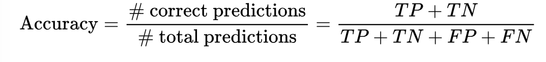
Accuracy

• What percentage of all observations was correctly

  categorized?

• Higher is better :)

• Doesn’t work with imbalanced problems

• measures the overall correctness of a model's predictions, representing the ratio of correct predictions to the total number of instances

• Accuracy = (True Positives + True Negatives) / (True Positives + True Negatives + False Positives + False Negatives). 

• If a model predicts the sentiment of 100 tweets and 85 of those predictions are correct, the accuracy is 85/100 = 85%. 

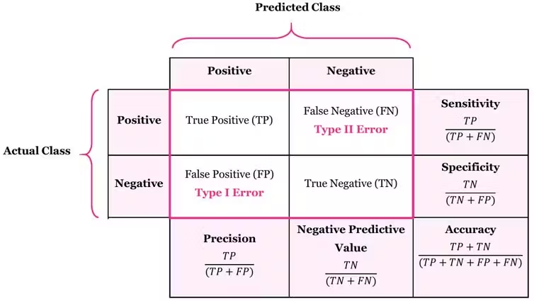
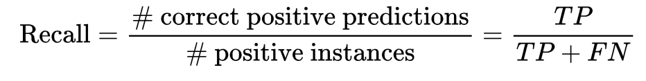
Recall

• Recall (Sensitivity or True Positive Rate) - for all

  actual yes, how often does it predict yes?

• TP / (TP + FN)

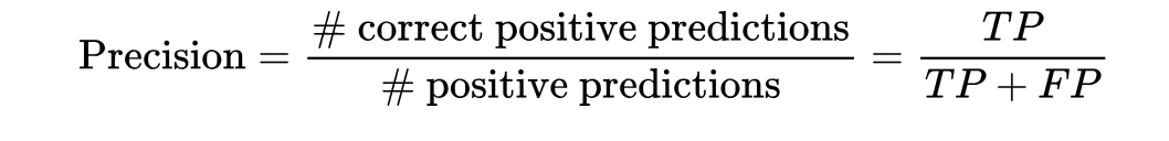
Precision

• when it predicts yes, how often is it

  correct?

• for all predicted yes, how often is it

  correct?

• TP / (TP + FP)

Regularization

• Want to find the optimal model without over- or

  underfitting.

• Regularization adds a “penalty term” to the loss

  function that shrinks the coefficients toward zero,

  simplifying the complexity of the model and

  identifying less important predictors.

• 3 Types

  • L1 (Lasso)

  • L2 (Ridge)

  • Elastic Net (combo)

LASSO (L1)

• Lasso - Least absolute shrinkage and selection

  operator

• Lasso is good for eliminating useless features

  since it can change the weights/coefs to zero.

• Helps reduce dimensionality

• Not good with small datasets

Ridge (L2)

• Penalizes large weights, but doesn’t eliminate

  them, so all features contribute

• Works with well with smaller sets since it keeps all features

Elastic Net (L3)

• Combination of the L1 and L2, a hyper parameter

  determine how much each regularization factor

  contributes. Note, we have two hyperparameters,

  (α and λ).

KNN Classification

• Supervised Learning

• Generally used for classification, but can also do

  regression

• Example of instance-based learning, doesn’t train

  or build a generalized internal model, but stores

  instances of the training data.

• Requires a lot of RAM

• Classify new item based on majority of the K

  neighbors.

• Hyperparameter K determines the number of

  neighbors, optimal choice of K is very data

  dependent

• Large K take a lot of computational power

• Distance-based algorithms, like KNN, must use

  properly scaled data.

• Use Standardization for scaling.

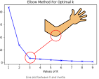
Elbow Method

graphs the total inertia of the clusters against values of \(k\) and chooses the \(k\) for which the curve levels off. Since increasing \(k\) also increases model complexity, the elbow method finds the \(k\) with the best tradeoff between complexity and inertia.

Grid Search

• Grid search is a method for finding the best hyperparameters for a machine learning model by systematically evaluating all possible combinations of hyperparameters within a predefined grid.

• How to:

  1. Choose model

     1. model = ElasticNet()

  2. Choose parameters

     1. param_grid = {‘alpha’:[0.1,2,5,10,50,100], ‘l1_ratio’:[.1,.5,.7,.95,.99,1]}

  3. Import needed libraries

     1. from sklearn.model_selection import GridSearchCV

  4. initialize GridSearch

     1. gridModel = GridSearchCV(estimater=model, param_grid=param_grid, scoring=‘neg_mean_squared_error’, cv=5, verbose=2)

  5. fit model

     1. gridModel.fit(X_train, y_train)

Standardization

• Center data with mean = 0 and standard deviation = 1

• Data is normally distributed

• Some outliers

• Linear/Logistic regression preform better with this.

Normalization

• Scale data to a fixed range, usually [0-1]

• Data is not normally distributed

• No extreme outliers

• Distance-based models (KNN, K-Means work better with

  normalized data

F1

• This is a weighted average of recall and precision.

Cross Validation

uses different subsets of the data for model training and model testing. Reserving a subset of the data for testing purposes allows fitted models to be evaluated without risk of bias. Cross-validation can be used to fine-tune a model's hyperparameters or choose between competing models.

Stratified cross-validation sets

evenly split, or balanced, for all levels of the output feature. In classification, stratification ensures that each cross-validation subset represents the class proportions in the total dataset. In regression, stratified samples are generated so that the descriptive statistics for each subset are about equal. Stratification is important when a given class or value is rare or when the fitted model depends on the class proportions.

k-fold cross-validation

splits a training set into \(k\) non-overlapping subsets, called folds. Each of the \(k\) subsets is used as validation data in one cross-validation run, with the remaining \(k-1\) subsets used for model training. Since cross-validation is performed multiple times, k-fold cross-validation can be used to measure the variability of parameters and performance measures. k-fold cross-validation may be used to select possible hyperparameter values or measure how sensitive a model's performance is to the training/validation split. Using more folds is computationally expensive, so 5-10 folds are recommended.

Leave-one-out cross-validation

(LOOCV) holds out one instance at a time for validation, with the remaining \(n-1\) instances used to train the model. Leave-one-out cross-validation is useful for identifying individual instances with a strong influence on a model. Leave-one-out cross-validation can be thought of as k-fold cross-validation with \(k = n\).

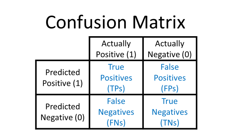
Confusion Matrix

is a table that summarizes the combinations of predicted and actual values. For binary classifiers, a confusion matrix is a table with two rows and two columns and gives the number of true positives, true negatives, false positives, and false negatives.

A true positive (TP) is an outcome that is correctly predicted as positive.

A true negative (TN) is an outcome that is correctly predicted as negative.

A false positive (FP) is an outcome that is predicted as positive but is actually negative.

A false negative (FN) is an outcome that is predicted as negative but is actually positive.

Imputation

group of techniques used in machine learning to replace missing values in a dataset with a reasonable estimate.

Feature Engineering

the process of selecting, manipulating, and transforming raw data into features that can be used in machine learning models to improve their accuracy and performance

Linear Regression

• Supervised Learning

• Use features and labels (X) to be able to predict a future outcome (y) based on unseen features

• Think “line of best fit”, assumes a linear relationship between features and labels (outcomes). EDA will confirm this early.

• Y = mx + b (m = slope, b = intercept)

• Outcome is a quantity/continuous value

• PRO: runs fast, no/little tuning required, highly

  interpretable and well understood. It lets us

  understand the relationship between outcome

  and importance of given features.

  • CON: Main drawback, unlikely to produce the best

  predictive accuracy compared to other modes

  since it assumes an underlying linear relationship

  between the features and the response value.

Univariate Regression

• we are trying to predict a single value

Multivariate Regression

• we are trying to predict a multiple value

Linear Regression (Simple)

models or predicts the output feature based on a linear relationship with only one input feature, y^=w0+w1⁢x. The weights w0 and w1 are the estimated y-intercept and slope.

Residual

the vertical distance between the

observed data value and the predicted value for the

instance by the linear model

Linear Regression (Polynomial)

xtends the simple linear model to include all p input features for predicting the output feature and takes the form y^=w0+w1⁢x1+w2⁢x2+...+wp⁢xp, where wj is the weight corresponding to the jt⁢h input feature for j=1,2,...,p. The weights wj represent the average effect on the output feature for a one-unit increase in xj, holding all other input feature values fixed.

KNN Regression

predicts the value of a numeric output feature based on the average output for other instances with the most similar, or nearest, input features. The k nearest instances, or neighbors, are identified using a distance measure with the input features. The average value of the output feature for the k nearest instances becomes the prediction. The k-nearest neighbors regression prediction is a numeric value compared to k-nearest neighbors for classification that predicts a class.

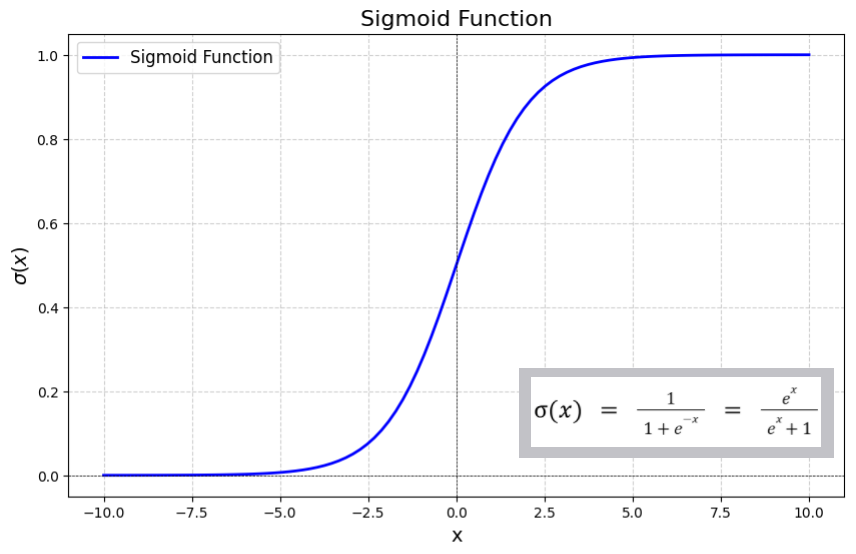
Logistic Regression

• Despite the name it’s not regression, but

  classification

• This classification yields membership probabilities

• Binary classification is the default

• Uses the sigmoid function to fit the data rather

  than a straight line

• This yields values 0 to 1 indicating membership

  probability of for a given class

Sigmoid Function

Ordinal Data

• implied order - can use integer encoding

Integer Encoding

• the process of converting categorical data (like text labels) into numerical values, typically integers, for easier processing by algorithms

• Mexico = 1, USA = 2, Canda = 3

one-hot encoding

• each category in a categorical feature is converted into a binary vector that has a length equal to the number of unique categories in the feature.

• male = 100, female = 010, child = 001

Dummy Encoding

• each category is assigned a unique binary vector with a length that is one less than the number of categories.

• male = 10, female = 01, child = 00

Nominal Data

• no inherent order - OHE or Dummy

Artificial Intelligence

Computers and programs to mimic human problem solving and decision making capabilities

Machine Learning

• Self-learning algorithms to derive knowledge from data in order to predict outcomes or organize data

• Semi-automated extraction of knowledge from data. I.e., it learning from examples and experience

• Sophisticated pattern matching

Regression

• Used to predict a quantity/continuous value

  • E.g., predict cost of a house based on location, # of rooms,

  square footage etc.

Model Evaluation

process of using metrics to assess how well a supervised machine learning model's predictions match observed values.

Classification Metric

• quantifies the predictive performance of a classifier by comparing the model's predictions to the observed classes.

• used to evaluate and compare fitted classification models.

• Common classification metrics include accuracy, precision, recall, confusion matrices, and kappa.

Accuracy

a classifier is the proportion of correct predictions

Precision

a classifier is the proportion of correct positive predictions

Recall

a classifier is the proportion of correctly predicted positive instances

F1-score

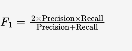
The harmonic mean of precision and recall. The harmonic mean is the reciprocal of the arithmetic mean of the reciprocals.Ex: For two numbers A and B, the harmonic mean is: ((A⁻¹+B⁻¹)/2)^-1

Fb-score

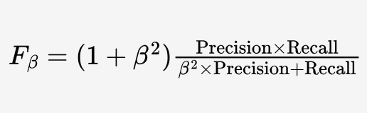
A weighted harmonic mean of precision and recall where β adjusts the tradeoff of importance between precision and recall. The precision has more importance when β<1, Fβ=F1 when β=1, and the recall has more importance when β>1.

Kappa

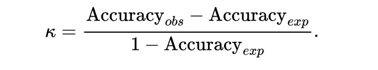
The metric kappa (κ) compares the observed accuracy of a classifier, Accuracy_o⁢b⁢s, with the expected accuracy, Accuracy_e⁢x⁢p, of a random chance classifier.

Model Selection

the process of identifying the best model from a set of fitted models. Model selection may be based on performance metrics, model interpretability, or model assumptions. Good models have:

• Strong performance. Ex: High accuracy, low mean squared error.

• Consistent performance. Ex: Models perform similarly during cross-validation or across multiple training/validation/testing splits.

• Reasonable assumptions. Ex: No model assumptions are seriously violated.

Models with low bias and variance models with high bias or high variance.

Cross-Validation

• tool for model selection, since each potential model is trained and validated across multiple splits. A good model should have strong performance metrics with low variability from one cross-validation split to the next.

• The same cross-validation splits should be used on each model to avoid bias.

1. Define a set of cross-validation splits.

2. Train and validate all potential models on every split.

3. Compare performance metrics on the validation sets using descriptive statistics or summary plots.

Model Tuning

the process of selecting the best hyperparameter for a model using cross-validation.

Tuning Grids

list of hyperparameter values to evaluate during model tuning. Tuning grids typically include between two and ten values of each hyperparameter. Grid values may be equally spaced, randomly selected, or chosen based on context.

Ex: The elastic net regression parameter λ adjusts the regularization method used. When λ is close to 0, the elastic net model is close to ridge regression, and λ near 1 is close to LASSO regression. So, a reasonable tuning grid for λ may be [0.0, 0.1, 0.5, 0.9, 1.0].

Multistage Model Tuning

finds the optimal parameter in multiple stages by refining the tuning grid after each stage and evaluating the refined grid on a new set of cross-validation folds. If a precise hyperparameter value is required, multistage tuning should be used.

Optimal Hyperparameter

hyperparameter that performs well in cross-validation. Depending on the performance metric and cross-validation strategy, several hyperparameters may be good fits. Often no single optimal hyperparameter exists, and several hyperparameter values may be acceptable.

Validation Curves

plot the mean cross-validation scores for each hyperparameter value tested in model tuning. Validation curves are useful for detecting overfitting: Hyperparameters that are overfitted will have high training scores and low validation scores. Optimal hyperparameters will perform well on the training sets and the validation sets.

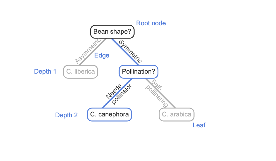
Tree

a hierarchical structure with no loops made up of two objects: nodes and edges.

Edge

is a directed link from a parent node to a child node. Most nodes in a tree have one parent node and multiple child nodes.

Root Node

the node with no parent node.

leaf

node that has no outgoing edges to child nodes.

depth

the number of edges that must be followed to reach that node from the root node.