Chapter 11 - Quasi-experimental designs and Applied Research

• Know the difference between a true experiment and a quasi-experiment

  • Influence of subject and other non-manipulated IVs 

  • Difference in conclusions that can be drawn

• Quasi-experimental designs have many of the characteristics of experiments, but lack the required manipulation of the IV (typically because random assignment was not used)

• Influence of Subject & Non-Manipulated IVs

  • True Experiment:

    • Controls for subject differences (e.g., age, IQ) via randomization.

    • Example: Randomly assigning patients to therapy vs. control groups.

  • Quasi-Experiment:

    • Subject variables (e.g., gender, trauma history) cannot be controlled, risking bias.

    • Example: Comparing PTSD symptoms in veterans vs. non-veterans (pre-existing groups).

• Difference in conclusions:

  • The conclusions that can be drawn are from Quasi Experimental designs cannot be causal

  • But, due to the high amount of control that is used in Quasi Experimental disgns, the degree of confidence of the findings tends to be higher than with studies with less rigor

What is the purpose of applied research? How does that differ from basic research? How are the two related to one another?

• Applied Research: Focused on defining and understanding a particular problem, with the hoped-for goal of solving that problem

• Basic research: is research for the purpose of expanding our general wealth of knowledge

• Related to one another by:

  • 1. Shared Goal:
    Both contribute to the "general fund of knowledge" in psychology by advancing understanding of human behavior, cognition, and emotion.

    2. Complementary Roles:

    • Basic Research:

      • Purpose: Expands theoretical knowledge (e.g., How does memory work?).

      • Example: Studying how sleep deprivation affects attention in a lab.

    • Applied Research:

      • Purpose: Solves practical problems (e.g., How can we improve shift workers’ alertness?).

      • Example: Testing a new caffeine-based alertness aid for nurses.

    3. Cyclical Relationship:

    • Basic research → Provides theories/tools for applied work.

    • Applied research → Identifies new questions for basic science.

      • Example: Discoveries about memory (basic) inform Alzheimer’s treatments (applied), which then reveal gaps in memory theory (basic).

    4. Mutual Dependence:

    • Without basic research, applied work lacks foundational principles.

    • Without applied research, theories may remain untested in real-world contexts.

Review the examples of applied research from lecture/slides; they provide good illustrations of how laboratory techniques can be used to solve ‘real world’ problems

• Ex 1: Walter Miles’ measurement of reaction time for the Stanford Football team’s offensive line members

  • Invented a “multiple chronograph” as a way to simultaneously measure all 7 members’ times

  • Measured other factors related to the players’ “charging time”

• Although his apparatus was not widely used, his work is a good example of a practical application of laboratory techniques to address real-world problems

• Ex 2: Hollingworth and Coca-Cola

  • In 1911, Coca-Cola was worried that they may lose their primary product due to one of its ingredients, which could run afoul of the recently passed Pure Food and Drug Act

    • That “dangerous ingredient” was caffeine 

      • It was considered to be addictive, and to mask the biological need to rest

    • The company went to court to defend its product, and research from the Hollingworths 

      • They were hired to evaluate the cognitive and behavioral effects

      • They also insisted that they could publish the results of their work, regardless of how it turned out

  • Lasted over a month

  • Involved multiple measurements, including reaction time, motor coordination, and more

  • N = 16

  • Used counterbalancing, testing each subject multiple times

  • Used a placebo control (sugar pills vs caffeine pills, at 3 different dosage levels)

  • Used a double-blind procedure

  • Results:

    • Results were complex, given the number of measures, dosages, etc.

    • Basically, found no detrimental effects of caffeine, except at higher dosages when given at the end of the day (some participants had some difficulty sleeping)

    • Coca-Cola was allowed to keep their product as it was

    • The case was actually dismissed for reasons other than the results of their study

• Know what a non-equivalent control group design is. 

  • Why do we assume the groups are not equivalent?

  • Why do some studies have to be non-equivalent?

  • What are the data of interest?

  • How do they help us rule out explanations for results?

• Non-equivalent control group design: In these designs, the groups are considered to not be equivalent at the start of the study AND they also experience difference conditions within the study itself

  • 1. Why Assume Groups Are Not Equivalent?

    • No Random Assignment: Participants are grouped based on pre-existing conditions (e.g., schools, clinics, genders), so differences (e.g., prior knowledge, socioeconomic status) likely exist.

    • Example: Comparing test scores of students from two different schools—even if similar, unmeasured factors (teacher quality, resources) may vary.

  • 2. Why Must Some Studies Be Non-Equivalent?

    • Ethical/Practical Constraints: Random assignment is often impossible or unethical.

      • Ethical: Can’t randomly assign people to smoke vs. not smoke to study lung cancer.

      • Practical: Can’t randomize entire schools to test curriculum reforms.

    • Natural Experiments: Leverage real-world groupings (e.g., policy changes in one state but not another).

  • 3. How Do They Help Rule Out Explanations?

    By controlling for confounds through:

    • Pre-Test Measures: Compare baseline scores to assess initial group similarity.

    • Matching: Pair participants on key variables (e.g., age, IQ) to reduce bias.

    • Statistical Controls: Use regression to adjust for known differences (e.g., income).

    Example:

    • Study: Comparing PTSD symptoms in veterans (non-randomized group) vs. non-veterans.

    • Ruling Out Confounds: Measure pre-service trauma, education, and age to isolate military service’s impact.

  • 4. Data of Interest: Due to the fact that the groups may differ at the beginning of the study, the data of interest are typically the difference scores between observations, rather than the difference of the end score

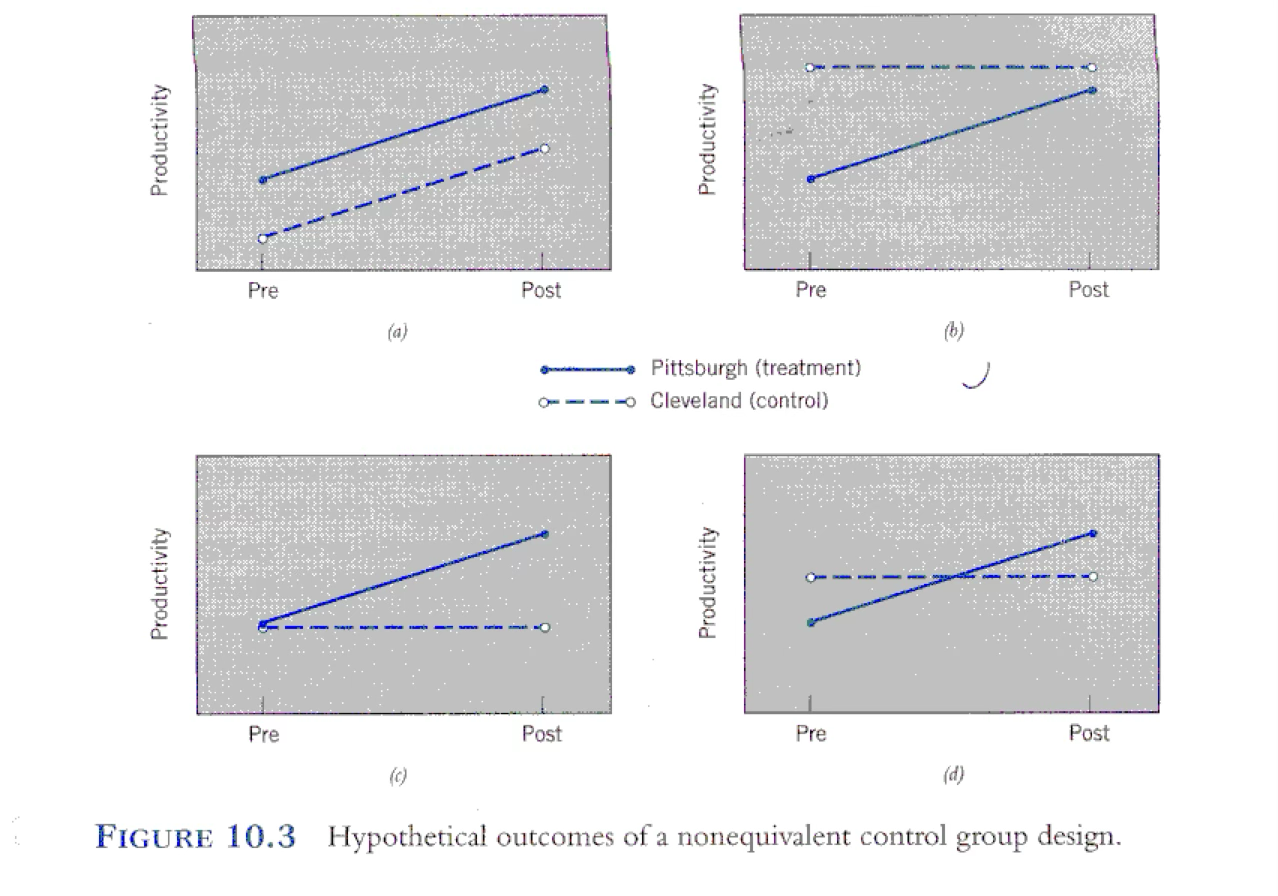
Cleveland vs. Pittsburgh example of non-equivalent control groups 

• Pittsburgh vs. Cleveland plants 

• Each plant’s productivity is measured for 1 month (pretest)

• In the Pittsburgh plant, they institute a flextime schedule (workers may concentrate all 40 hours in 4 days instead of 5)

• In the Cleveland plant, the workers keep to the traditional schedule (non-flextime)

• After 6 months productivity is measured again

• Possible outcomes:

  • a:  both groups improved at the same rate, suggesting that there was something happening at that time (history or maturation, for example) that affected everyone

  • b:  possibility of ceiling effect in the control group (nowhere to go), or regression to the mean in the treatment group (they started abnormally low)

  • c: this may show support for the effectiveness of flextime, but it’s also possible that history might have affected the treatment group’s scores (e.g. some event in only that city), or just knowing they’re in a study might have affected them

  • d: strongest support – the treatment group started lower, but surpassed the control group, helping to rule out regression

• How can the use of matching introduce potential problems? Also, regression effects?

1. Problems with Matching

Matching aims to make groups comparable by pairing participants on key variables (e.g., age, IQ), but it can introduce:

• Overmatching:

  • Matching on irrelevant variables reduces statistical power without improving validity.

  • Example: Matching on shoe size in a study of reading skills.

• Incomplete Matching:

  • Failing to match on unmeasured confounds (e.g., socioeconomic status, motivation) leaves bias.

  • Example: Matching students by school but ignoring parental involvement.

• Reduced Sample Size:

  • Discarding unmatched participants shrinks the sample, limiting generalizability.

• Artificial Similarity:

  • Forces equivalence on matched traits but ignores natural group differences.

---

2. Regression to the Mean (Regression Effects)

When groups are selected based on extreme scores, their subsequent measurements tend to move toward the average, creating false trends:

• Problem: Misinterpreting natural score changes as treatment effects.

• Example:

  • A school intervenes with the lowest-scoring students. Even without treatment, their scores may improve slightly (regressing toward the mean), falsely appearing as success.

• Solution: Use a control group to distinguish regression from true effects.

Examples that portray how matching can introduce potential problems as well as regression effects:

• Hypothetical example of reading level study:

  • A program is designed to improve reading skills in disadvantaged youths in a particular city

  • The target population has lower than average scores compared to the general population

  • To create a control group, a sample of children from a similar SES is found that matches the experimental group on reading level

    • By matching on low pretest scores, both groups were prone to regression to the mean—their scores would naturally improve toward the average over time, even without intervention.

      • What Happened:

        • Control group: Improved from 25 → 29 (regression effect).

        • Experimental group: Stayed at 25 (program may have prevented natural regression).

        • False Conclusion: The program "hurt" advancement, when in reality, it might have stopped scores from dropping further or simply had no effect.

  • Hypothetical result:

  • Experimental group:   25         Program           25

  • Control group:             25                                   29

  • Interpretation?

    • These results appear to suggest that not only isn’t the program effective, but it seems to hurt the children’s advancement

    • However, due to the procedure used, regression to the mean is likely affecting both group’s results.

• Head Start

  • 1. Head Start (Purpose?)

    • Program Goal: Provide early childhood education to low-income children to reduce achievement gaps.

    • Regression Risk: Children selected for Head Start often start with extremely low test scores (bottom of the distribution). Even without intervention, their scores may naturally regress toward the mean over time, creating a false impression of program success.

    • LBJ’s Vision: Head Start aimed to break the cycle of poverty through early education, nutrition, and family support.

    • Nixon’s Era: The Westinghouse study’s methodology was later criticized for regression artifacts and non-equivalent comparisons, but Head Start endured as a legacy program.

    2. Westinghouse Evaluation Project

    • Study Design: Evaluated Head Start’s effectiveness by comparing participants to non-participants.

    • Regression Problem:

      • Compared groups were non-equivalent (no random assignment).

      • Head Start children’s scores improved post-program, but this could partly reflect natural regression from their initial low baseline.

      • Control groups (less extreme scores) showed smaller gains, exaggerating Head Start’s apparent impact.

    3. “Fade-Out Effects”

    • Finding: Early academic gains from Head Start often diminished within a few years.

    • Link to Regression:

      • Initial "gains" may have been inflated by regression effects (extreme scorers naturally improving).

      • As scores stabilized near the mean, the program’s true long-term effects became clearer (and smaller).

    4. Why Misinterpretation by Politicians?

    • Overstated Claims: Politicians cited short-term improvements (potentially confounded by regression) as proof of success, ignoring fade-out.

    • Ignored Context: Failed to account for:

      • Non-equivalent groups (Head Start kids faced more systemic challenges).

      • Regression artifacts (natural score changes ≠ program efficacy).

Extra Credit Question: Who was the president when the Head Start program was started vs who was the president when it was evaluated?

• Start: Lyndon B. Johnson

• End: Richard Nixon

• What do interrupted time series designs add that other, simpler designs do not?

  • Review the anti-smoking campaign example

• Another type of quasi-experimental design

• Measures taken for an extended period before and after an event occurs that is expected to influence behavior

  • O1 O2 O3     E     O4 O5 O6

    • Where O = , E = 

• Allows for examination of pattern of behavior over time with reference to “event”

• Design allows researcher to rule out alternative explanations of an apparent change from pre- to post-test

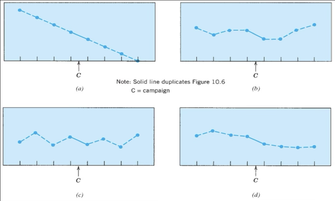
  • Example:  Effects of antismoking campaign on teenage smoking behaviors

    • Compare interpretation from pre- post-test design vs. interpretation from interrupted time series design

      • Top Left: no effect of campaign

        • Smoking was already going down before campaign was shown

      • Top right: no effect of campaign

        • Smoking was up & down but went up to its highest point after the campaign was shown

        • Effectiveness faded out

      • Bottom left:

        • As smoking rates were on a up and down before and after campaign

      • Bottom right:

        • This shows that the campaign had an effect because even though it was already on a downward decline there was a huge decline jump after the campaign

How can the addition of a control group (e.g. the Connecticut traffic fatality study) help us better understand results?

• Inclusion of control condition can help with interpretation

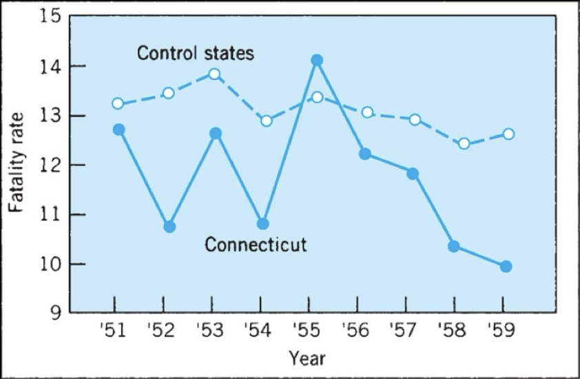
• In Connecticut Traffic Fatality Study:

  • The addition of a control group in the Connecticut traffic fatality study allowed researchers to account for potential confounding variables. For example, if traffic fatality rates were changing nationwide due to broader trends (like changes in vehicle safety, road conditions, or driving behaviors), comparing Connecticut to similar control states helps isolate the effect of any specific intervention or policy implemented in Connecticut. This way, we can better determine whether changes in Connecticut’s fatality rate were likely due to the intervention, rather than part of a general national trend.

What is meant by switching replications, and how does that help rule out alternative explanations for results?

• Switching replications

  • Vary the time at which the “event” or treatment is put into place

  • Ask yourself whether change can be directly tied to the event

    • Ex:

    • O1 O2 O3 E O4 O5 O6 O7 O8

      OR

    • O1 O2 O3 O4 O5 O6 E O7 O8

• Help rule out alternative explanations for results:

  1. History Effects (External Events):

     • If an unrelated event (e.g., a policy change) affects results, it would impact both groups when they switch roles, revealing the true treatment effect.

  2. Maturation/Regression Artifacts:

     • Natural changes (e.g., skill improvement over time) should appear in both groups when untreated, isolating the treatment’s impact.

  3. Selection Bias:

     • If Group A and Group B differ at baseline, the switch shows whether effects are consistent across groups or tied to pre-existing differences.

  4. Testing Effects:

     • Repeated measurements might influence behavior (e.g., test practice), but effects should appear in both phases, making the treatment’s role clearer.

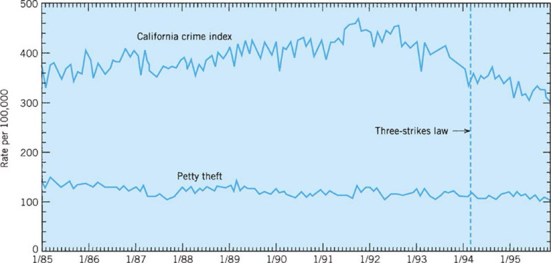
Why would measuring multiple variables (e.g. the 3 strikes and you’re out example) be a good thing?

1. Captures Complex Real-World Effects

Policies like "Three Strikes" (mandating life sentences for repeat offenders) have multidimensional impacts that single metrics miss. Measuring multiple variables allows researchers to assess:

• Crime rates (e.g., violent vs. property offenses).

• Incarceration costs (e.g., prison overcrowding, taxpayer burden).

• Social outcomes (e.g., recidivism, community trust in law enforcement).

Example: A study might find that while the policy reduces repeat offenses (strike 1), it also increases prison populations (strike 2) and disproportionately targets minorities (strike 3).

2. Rules Out Confounding Explanations

Single-variable studies risk spurious conclusions. Multiple measures help isolate causality:

• Did crime drop because of "Three Strikes" or other factors (e.g., economic growth, policing strategies)?

• Tracking unemployment rates, policing budgets, and demographic data alongside crime stats clarifies the policy’s true impact.

3. Balances Trade-Offs

Policies often have unintended consequences. Measuring multiple variables reveals:

• Cost-benefit analyses: Does the drop in crime justify soaring prison costs?

• Equity impacts: Are marginalized groups unfairly targeted?

Example: California’s "Three Strikes" law reduced felonies but led to life sentences for nonviolent offenders—a trade-off only visible by measuring sentencing patterns alongside crime rates.

4. Strengthens Generalizability

Context matters. Measuring variables like:

• Regional differences (urban vs. rural crime trends).

• Timeframes (short-term vs. long-term effects).
  ... ensures findings aren’t limited to one setting.

5. Informs Policy Adjustments

Policymakers need nuanced data to refine laws. For instance:

• If "Three Strikes" reduces burglaries but not homicides, states might exclude nonviolent crimes.

• If racial disparities are found, reforms could address sentencing biases.

E.g., Three strikes and you’re out policy in California

Know what Program Evaluation is, including its 4 purposes/phases

• Program evaluation: is a form of applied research that uses a variety of strategies to examine the effectiveness of programs designed to help people.

• A specific type of applied research

  • 4 major purposes

    • Needs Analysis = determine community and individual needs for programs

    • Formative Evaluative = assess whether program is being run as planned and if not implement change

    • Summative Evaluation = evaluate program outcomes

    • Cost-Effectiveness Analysis