Chapter 10 - Matrices

Matrices - in a nutshell (literally)

Matrix Basics

• Table of numbers only, in square brackets

• Named by usually capital letters

• Rows = horizontal, Columns = vertical

• Order = rows × columns (e.g. 2×3)

• Elements identified by row & column (like d₂,₃)

Types of Matrices

• Row matrix: single row

• Column matrix: single column

• Square matrix: equal rows & columns

Special Square Matrices

• Diagonal: only main diagonal has non-zero elements, such as

• 9 0 0 0

  0 4 0 0

  0 0 7 0

  0 0 0 3

• Identity: diagonal matrix with 1’s on diagonal, acts like 1 in multiplication, such as

• 1 0 0

  0 1 0

  0 0 1

• Symmetric: aᵢⱼ = aⱼᵢ, mirrored over main diagonal (pic)

• Triangular:

  • Lower = zeros above diagonal

  • 3 0 0 0

    5 2 0 0

    1 -4 7 0

    9 8 2 6

  • Upper = zeros below diagonal

  • 4 5 1 7

    0 3 9 2

    0 0 6 8

    0 0 0 5

• Summing: row or column matrix of all 1’s used to sum elements in rows or columns by multiplication such as

• 1

  1

  1

  1

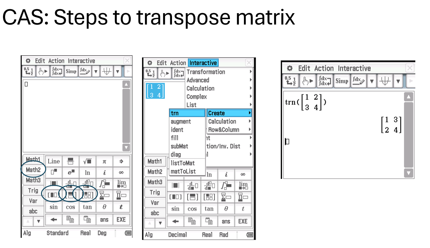
Transpose Matrix

• Transpose: swap rows and columns

• CAS tip: clear all variables after solving to avoid conflicts

Network Matrices

• Represent network with an n × n matrix (n = number of points)

• Element = 1 if two points are connected by a line

• Element = 0 if two points are NOT connected

• Rows and columns correspond to points (nodes)

• Matrix shows all connections clearly and simply

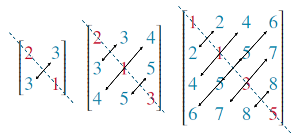
Constructing Matrices Using Element Rules (aᵢⱼ)

• Each element aᵢⱼ depends on row (i) and column (j) numbers

• Apply the given formula/rule to i and j to find each element

• Example 1 (Matrix A): aᵢⱼ = i + j

  • a₁₁ = 1 + 1 = 2

  • a₁₂ = 1 + 2 = 3

  • a₂₁ = 2 + 1 = 3

  • a₂₂ = 2 + 2 = 4

• Example 2 (Matrix B): aᵢⱼ = 2i - j

  • a₁₁ = 2×1 - 1 = 1

  • a₁₂ = 2×1 - 2 = 0

  • a₂₁ = 2×2 - 1 = 3

  • a₂₂ = 2×2 - 2 = 2

Matrix Addition & Subtraction

• Add or subtract by adding/subtracting corresponding elements

• Only possible if matrices have the same order (same size)

• Result matrix keeps the same element positions as originals

• Use CAS to make it easier!

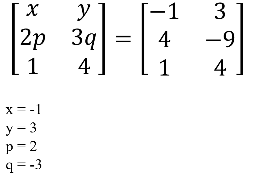
Matrix Equality

• Two matrices are equal if:

  • They have the same dimensions (order)

  • Every corresponding element is equal

• If dimensions differ, matrices can’t be added or compared for equality

• When given matrices with unknowns (like x, y, p, q), set corresponding elements equal to solve for variables

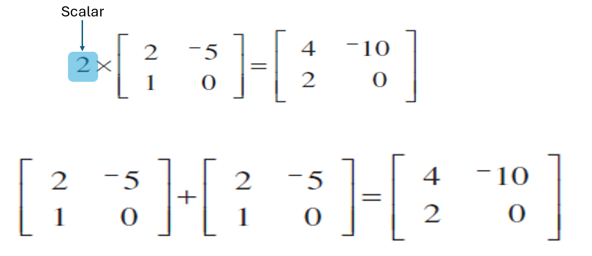
Multiplication by Scalar

• Multiply each element of the matrix by the scalar (number)

• Like distributing a factor across a bracket in algebra

• Keeps matrix size unchanged

• Same drill - use your CAS!

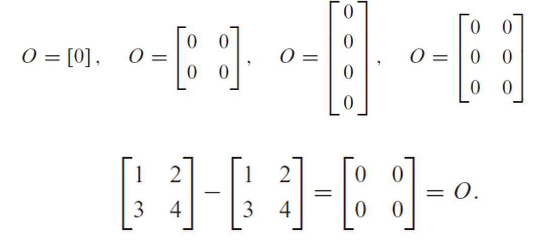
Zero Matrix

• A matrix with all elements zero

• Can be any order (size)

• Symbolized by O (capital letter O)

• Acts like zero in matrix addition (A + O = A)

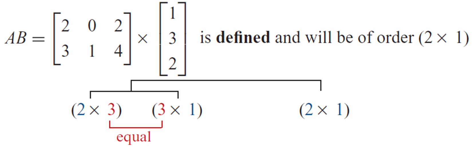
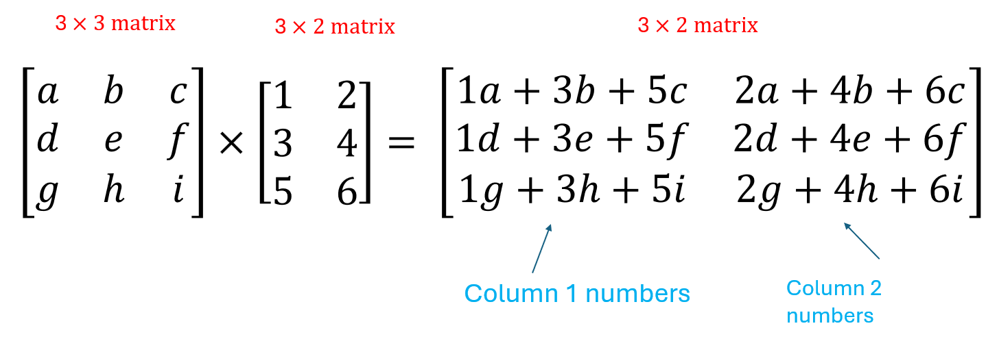
Matrix Multiplication Dimensions

• Multiply an m×n matrix by an n×q matrix

• Result is an m×q matrix

• Columns of 1st = Rows of 2nd (must match)

• Each element = sum of products of row i (1st matrix) × column j (2nd matrix)

• Result element goes in row i, column j of product matrix

Rules for Summing Rows & Columns

• Sum rows of an (m × n) matrix:
  Post-multiply by a (n × 1) column summing matrix (all 1’s)
  — Result is an (m × 1) matrix with row sums

• Sum columns of an (m × n) matrix:
  Pre-multiply by a (1 × m) row summing matrix (all 1’s)
  — Result is a (1 × n) matrix with column sums

Matrix Powers

• Raising a matrix to a power = multiplying the matrix by itself repeatedly

• NOT just raising each element to that power

• Example:

• [1 2; 3 4]^2 = [1 2; 3 4] × [1 2; 3 4]

  = [1×1 + 2×3 1×2 + 2×4

  3×1 + 4×3 3×2 + 4×4]

  = [7 10

  15 22]

• This is NOT equal to

• [1^2 2^2

  3^2 4^2] = [1 4

  9 16]

• Only square matrices (same rows and columns) can be raised to powers

• Because matrix multiplication requires the number of columns in the first matrix to match rows in the second

Properties of Multiplication of Matrices

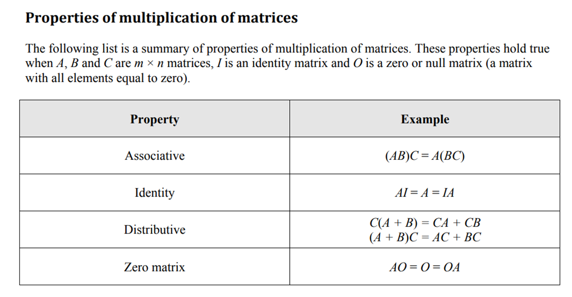
We have seen commutative property of multiplication does not hold.. AB ≠ BA!

Determinant of Matrix

For matrix

A = [a b

c d]

• Determinant:
  det(A) = ad – bc

• If det(A) = 0 → no inverse, matrix is Singular

• If det(A) ≠ 0 → inverse exists, matrix is Regular

Inverse Matrices

• Only square matrices with det(A) ≠ 0 have inverses

• For A = [a b

  c d]:

• A⁻¹ = (1/det(A)) × [ d -b

  -c a ]

• Steps:

  • Find det(A) = ad - bc (must ≠ 0)

  • Swap elements on main diagonal (a ↔ d)

  • Change signs of off-diagonal elements (b, c)

  • Multiply entire matrix by 1/det(A)

Special Properties of Inverse Matrices

• A⁻¹ is the inverse of matrix A

• Multiplying a matrix by its inverse gives the identity matrix:

  • A × A⁻¹ = I

  • A⁻¹ × A = I

• Identity matrix I acts like 1 in multiplication — no change

• Inverse perfectly undoes the matrix operation

Solving Matrix Equations

• Like solving linear equations but with matrix twists

• Order of multiplication matters — switching sides changes results

• No division for matrices

• Instead, multiply by the inverse matrix to “divide” and isolate variables

Solving Simultaneous Equations with Matrices

• Given system:
  2x + 3y = 13
  5x + 2y = 16

• Write as matrix equation:
  A × X = B
  where
  A = [2 3; 5 2]
  X = [x; y]
  B = [13; 16]

• Solve by finding X = A⁻¹ × B

• (Also can use CAS)

Simutaneous Equations with Matrices - No Solution Case

• If determinant of matrix A = 0, inverse does not exist

• Singular matrix = matrix with determinant = 0 * therefore no solution exists for singular. Any other matrix with determinant ≠ 0 has a solution(s).

• No unique solution for the system of equations

• Example:

• 3x + 2y = 9

  6x + 4y = 22

• Matrix form:
  A = [3 2; 6 4], X = [x; y], B = [9; 22]

• Since det(A) = 3×4 - 6×2 = 12 - 12 = 0, no inverse

• So, X = A⁻¹ × B is undefined → no unique solution

Binary Matrices

• A binary matrix contains only 0s and 1s

• Used for networks, logic, and digital systems

• Special binary matrices include:

  • Summing matrices (all 1s in a row or column)

  • Identity matrices (1s on diagonal, 0s elsewhere)

  • Zero matrices (all 0s)

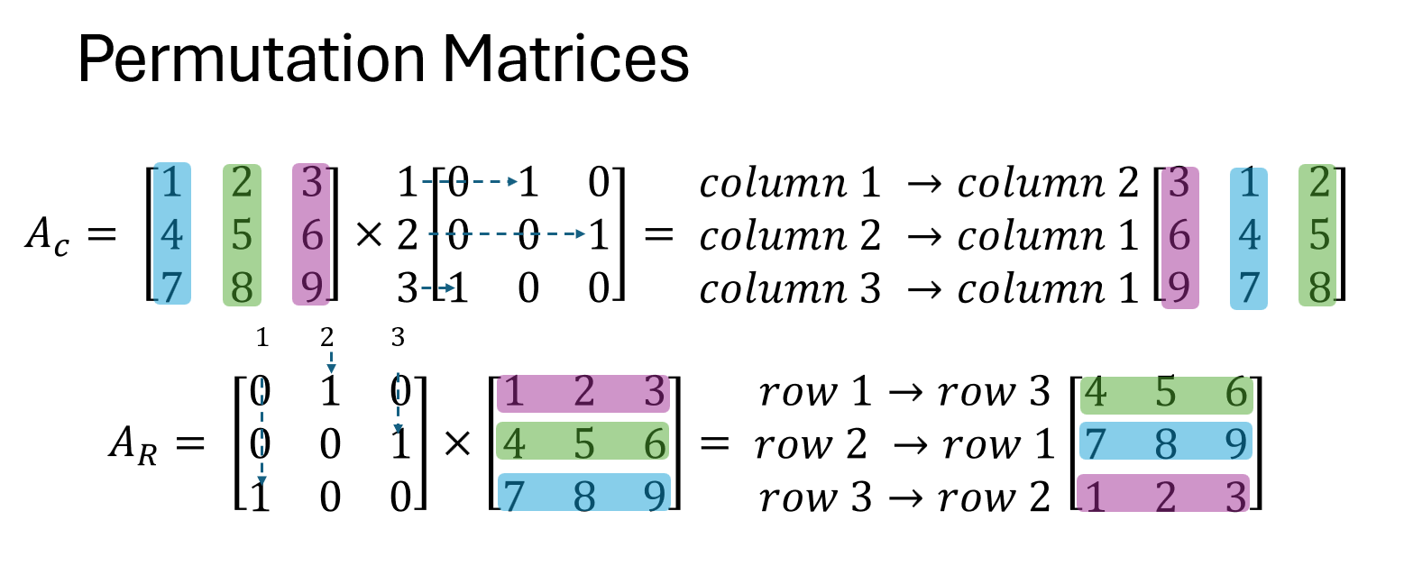
Permutation Matrices

• A square binary matrix

• Exactly one 1 per row and per column

• Used to rearrange rows or columns of another matrix

• Pre-multiply → row permutation

• Post-multiply → column permutation

• TIP: For XPⁿ=X for n is the smallest, n = amount of letters shuffled e.g., 2 letters shuffled = squared.

Inverses:

• Every permutation matrix has an inverse

• The inverse is just the transpose:

  • P⁻¹ = Pᵀ

• Easy to reverse — just flip rows and columns!

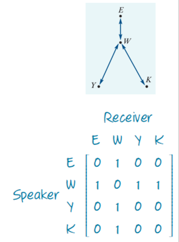
Communication Matrices

• Communication matrix: square binary matrix showing who can talk to who

• Rows = sender, columns = receiver

• 1 = direct communication possible, 0 = not possible

• Row sum = how many people someone can talk to

• Column sum = how many people someone can hear from

Why use both matrix & network diagram?

• Matrix shows data clearly and allows math (like squaring)

• Network diagram shows visual relationships (easy to see gaps)

• Squaring the matrix reveals two-step communication paths

Two-Step Communication Matrix

• Created by squaring the communication matrix → C²

• Shows indirect communication (via an intermediary/translator)

• 1 in C²[i,j] = person i can reach person j in two steps

• Leading diagonal = redundant links (person reaching themselves – not useful)

Example Insight

• C[4,1] = 1: Wong can directly send message to Eva

• C²[4,1] = 0: No two-step path from Wong to Eva — already direct, no need for intermediary

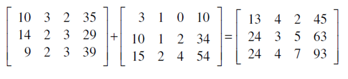
Total Communication Links (T = C + C²)

• T = C + C²

• Adds direct (1-step) and indirect (2-step) communication

• Each element in T[i,j] tells how many ways person i can reach person j

• Helps analyse the full reachability of each person in the system

• T shows who can talk, who needs help to talk, and who’s left out!

Redundant Communication Links

• Redundant = extra, not needed, adds no new info

• In matrix powers:

  • C³, C⁴... often repeat paths already found in C + C²

• Only useful in very large or complex networks

• For small systems, powers beyond 2 are usually redundant

Dominance Matrix

• Used in round-robin tournaments

• Row = winner, Column = loser

• Entry is 1 if row player beat column player

• Diagonal is 0 (no self-wins → redundant)

• Opposite positions (i,j) and (j,i) are mutually exclusive

• Row sum = total wins by that player

• It’s the scoreboard of the battlefield — no ties, no mercy!

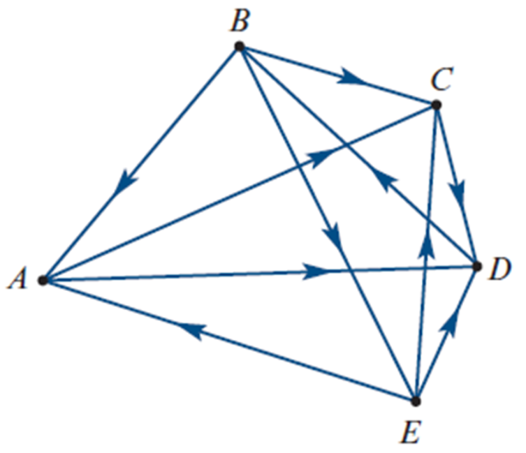
Dominance Network Diagrams

• Visual map of who beats who in a competition

• Arrow direction: points from winner (dominant) → loser (non-dominant)

• Shows hierarchy of strength or skill

• Example:

  • Anna → Cas, Di

  • Brigit → Anna, Cas, Emma

  • Cas → Di

  • Di → Brigit

  • Emma → Anna, Cas, Di

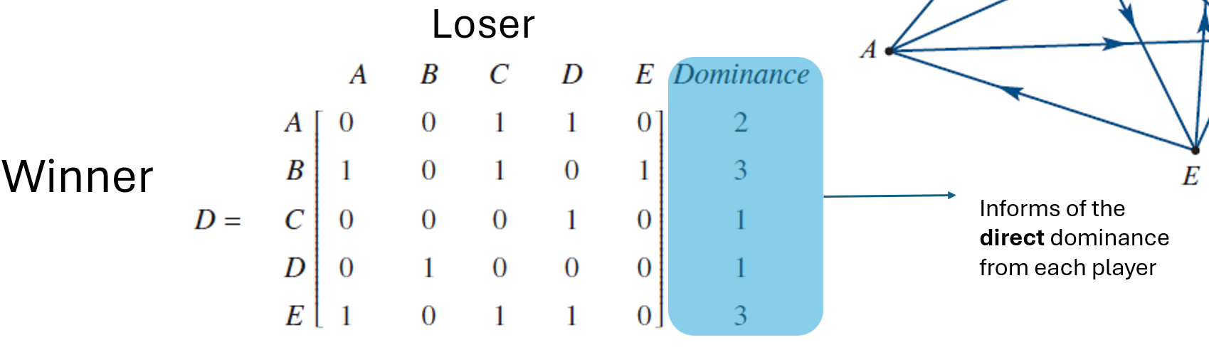
One-step Dominance Matrix

• Captures direct wins only — who beat whom in one step

• Rows = winner (dominant)

• Columns = loser (non-dominant)

• Entry = 1 if row player beat column player, else 0

• Simplifies dominance network into a neat matrix form

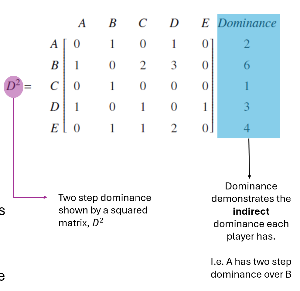
Two-step Dominance

• Represents indirect dominance via one intermediary

• Found by squaring the one-step dominance matrix

• Example: A beat B, who beat C → A two-step dominates C

• Helps break ties when players have equal direct wins

• Reveals deeper hierarchy beyond immediate wins

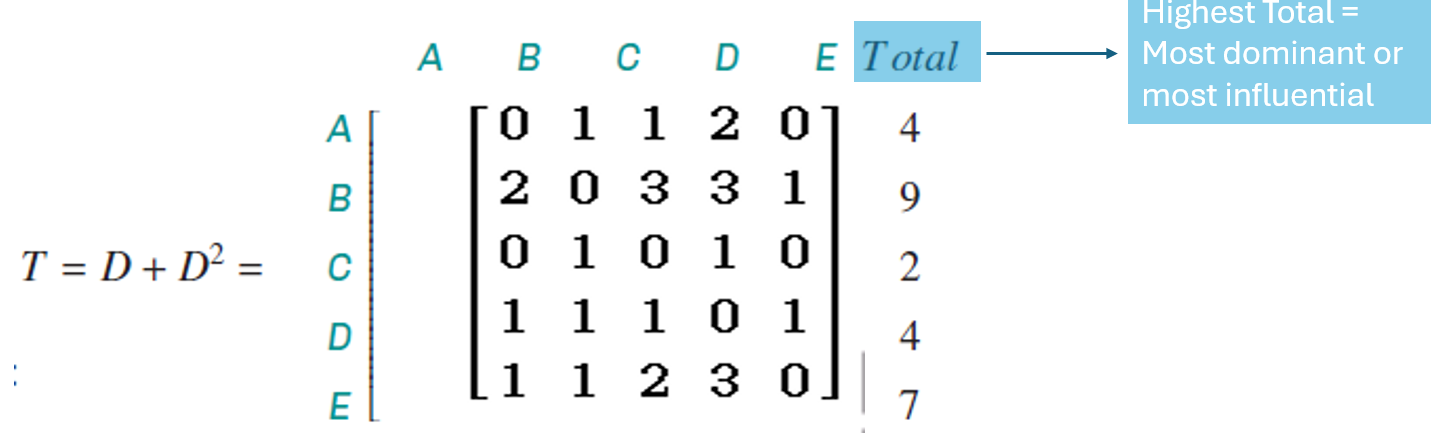
Total Dominance

• T = D + D² combines one-step and two-step dominance

• Adds direct wins and indirect influence into one matrix

• Sum of each row = total dominance score of that individual

• Highest score = most dominant player

• Reveals the full picture: immediate victories + power through others