ACTEX SRM Study Manual - Chapter 8 - Decision Trees

decision tree, aka tree-based models

non-parametric alternative approach to regression in which we will segment the predictor space into a series of non-overlaping regions of relatively homogeneous observations

predictor space

the set of all possible combinations of predictor values (or levels)

section 8.1 starts here

single decision trees

node

a point on a decision tree that corresponds to a subset of the predictor space. all training observations whose predictor values belong to that subset will live in the same node

what are the three types of nodes

1. root node

2. internal node

3. terminal nodes (aka leaves)

root node

node at the top of the decision tree representing the full predictor space and containing the entire training set

internal nodes

tree nodes which are further broken down into smaller nodes by one or more splits (includes the root node)

terminal nodes (aka leaves)

nodes at the bottom of a tree which are not split further and constitute an end point

branches

lines connecting different nodes of a tree

how to use decision trees for prediction

use the classification rules to locate the terminal node in which the observation lies. then predict the observation by using the sample response mean in that terminal node

recursive binary splitting is a top-down, greedy approach

top-down means that we start from the top of the tree and go down and sequentially partition the predictor space in a series of binary splits

greedy is a technical term meaning that at each step of the tree-building process, we adopt the best possible binary split that leads to the smallest RSS at that point, instead of looking ahead and selecting a split that results in a better tree in a future step

first step of recursive binary splitting

aka, choose Xⱼ and s ∋ the sum of the two branches RSS' are minimized

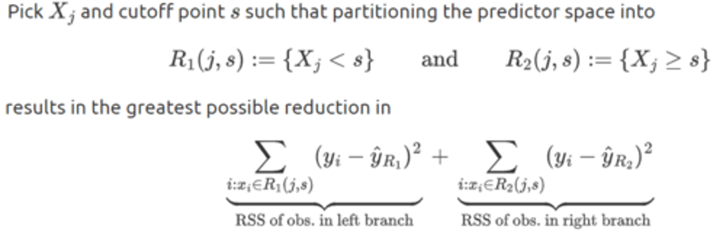
sbsequent splits of recursive binary splitting

after the first split there will be two regions in the predictor space. next, we seek the best predictor and the corresponding cutoff point for splitting one of the two regions (not the whole predictor space) in order to further minimize the RSS of the tree

stopping criterion of recursive binary splitting

each splits operates on the results of previous splits until we reach a stopping criterion, e.g., the number of observations in all terminal nodes of the tree falls below some pre-specified threshold, or there are no more splits that can contribute to a significant reduction in the node impurity

why do we prune a tree?

recursive binary splitting often produces a decision tree that overfits. we want to create a mode compact, interpretable, and useful tree

the size of a tree is measured by

the number of terminal nodes the tree has (comparable to the number of (non-zero) coefficients in a GLM

as the size of a decision tree increases,

the tree becomes harder to interpret and liable to produce predictions with a high variance

(unstable predictions can be the result of the final split being based on a very small number of training observations)

cost complexity pruning (aka weakest link pruning)

for each value of 𝛼, we find a subtree T𝛼 that minimizes

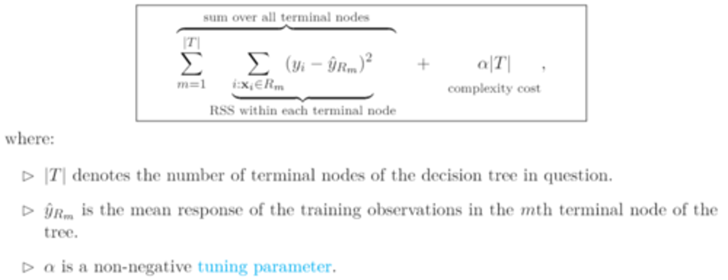
as 𝛼 increases

the penalty term becomes greater and the tree branches are snipped off starting from the bottom of T₀ to form new, larger terminal nodes.

the fitted tree T𝛼 shrinks in size

bias² increases

variance decreases

a decision tree for predicting a quantitative response is called a (regression/classification) tree, while a decision tree for predicting a qualitative response is called a (regression/classification) tree

a decision tree for predicting a quantitative response is called a regression tree, while a decision tree for predicting a qualitative response is called a classification tree

what are the two differences between a classification tree and a regression tree?

1. predictions in a classification tree use the response mode instead of the response mean

2. we use the classification error rate instead of the RSS as a goodness-of-fit measure

classification error rate (qualitative)

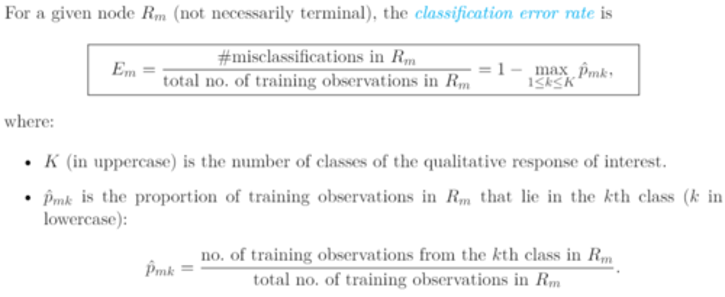
max 1≤k≤K p̂ₘₖ aka the highest class proportion

the proportion of training observations belonging to the most common level of the response variable in Rₘ

the lower the value of Eₘ, the higher/lower the value of max 1≤k≤K p̂ₘₖ

the lower the value of Eₘ, the higher the value of max 1≤k≤K p̂ₘₖ, and the more concentrated or pure the observations in Rₘ in the most common class

a large Eₘ is an indication that the observations in Rₘ are

impure

criticism against the classification error rate

it is not sensitive enough to node purity in the sense that it depends on the class proportions through the maximum

gini index and entropy

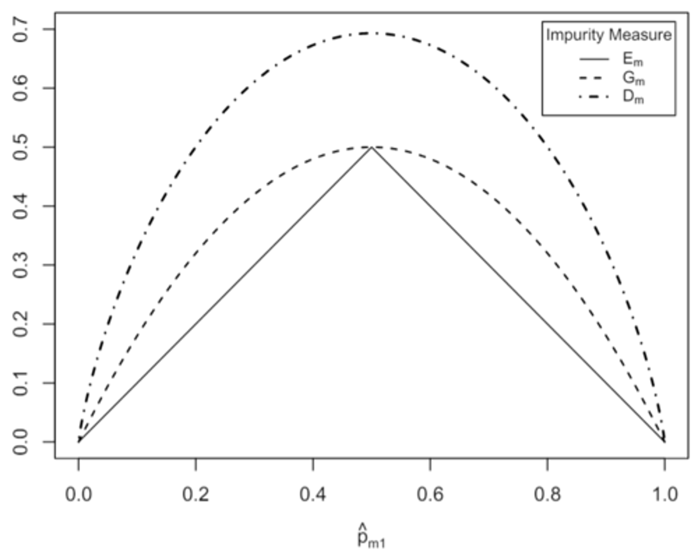
the larger the value the more impure or heterogenous the node

gini index of a given node Rₘ is defined as

which is a measure of total variance across the K classes of the qualitative response in that node

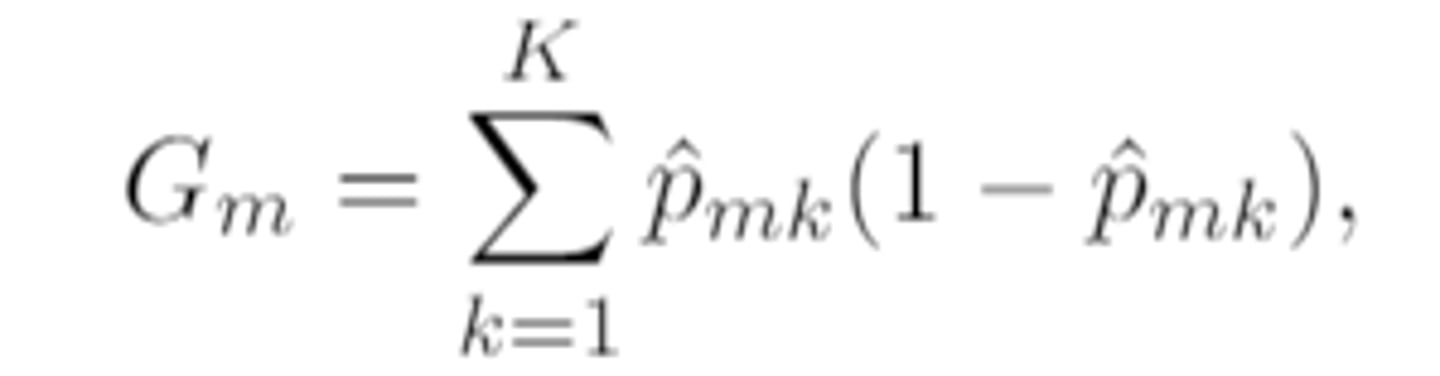
variance of a bernoulli RV

p̂ₘₖ(1-p̂ₘₖ)

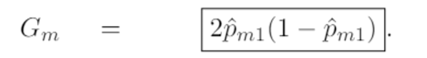
expanded gini index

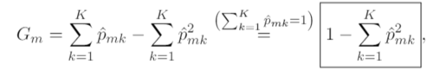
in the special case of K=2 (i.e. the categorical response is binary), the gini index silplifies to

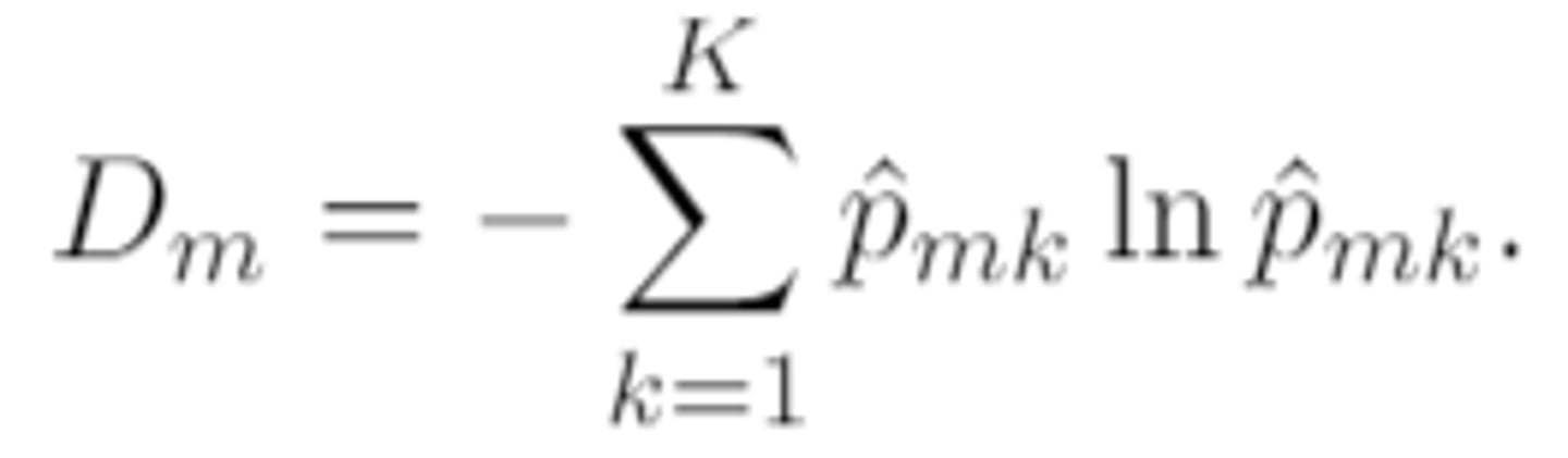
entropy (aka cross-entropy)

behavior of the classification error rate, gini index, and entropy considered as a function of p̂ₘ₁ when K=2

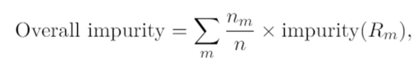
overall impurity for a binary split that produces two "child" nodes

take the weighted average of the classification error rates/gini indices/cross-entropies of different nodes, with the weights given by the number of observations

overall impurity for a classification tree with m (≥2) terminal nodes

overall impurity when the impurity measure is the classification error rate simplifies to

sum of # of misclassifications in all terminal nodes / n

advantages of trees over linear models

1. easier to explain and understand

2. reflect more closely the way humans make decisions

3. more suitable for graphical reporesentation, which makes them easier to interpret

4. can handle predictors of mixed types (i.e. qualitative and quantitative) without the use of dummy variables, unlike GLMs

disadvantages of trees compared to linear models

1. do not fare as well in terms of predictive accuracy

2. can be very non-robust (a miniscule change in the training data can cause a substantial change in the fitted tree)

section 8.2 starts here

ensemble trees

ensemble methods allow us to

hedge against the instability of decision trees and substantially improve their prediction performance in many cases

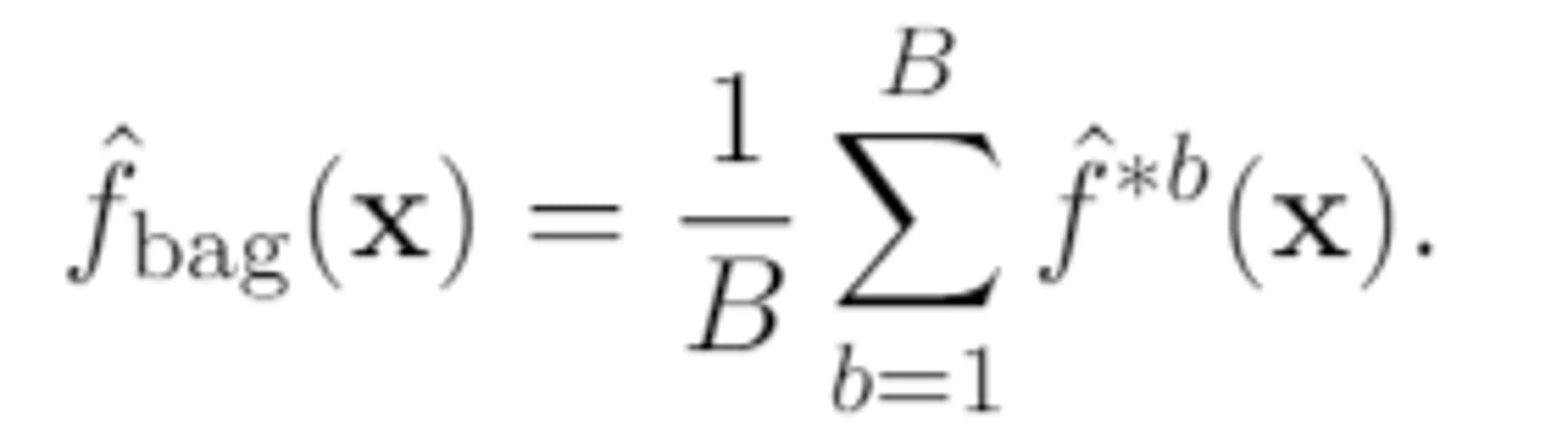
bagging (aka bootstrap aggregation)

based on the bootstrap, which involdes generating additional samples by repeatedly sampling from the existing observations with replacement to improve the prediction accuracy of a tree-based model

if the response is quantitative, then the overall prediction is

the average of the B base predictions (which are also numeric)

if the response is qualitative, then the overall prediction is

calculated by taking the "majority vote" and picking the predicted class as the class that is the most commonly occurring among the B predictions

pros of bagging (relative to a single tree)

variance reduction (bias however does not reduce by bagging)

cons of bagging (relative to a single tree)

1. less interpretable

2. takes considerably longer to implement

variable importance score

provides an overall summary of the importance of a variable.

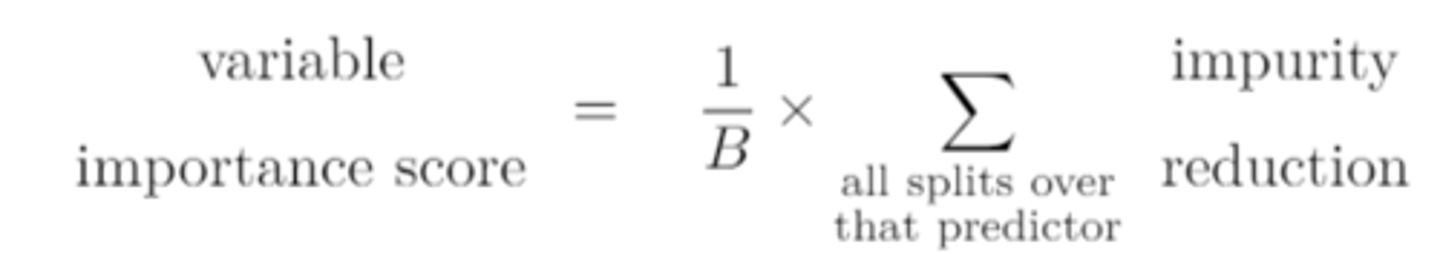
the larger/smaller the importance score of a predictor, the larger the average reduction in impurity due to that predictor, and the more "important" it appears

the larger the importance score of a predictor, the larger the average reduction in impurity due to that predictor, and the more "important" it appears

random forests

these are improved versions of bagging that seek to further improve on the prediction performance of an ensemble tree model.

while bagging involves averaging identically distributed and often correlated trees, random forests make the bagged trees less correlated and enhance the variance reduction via an additional degree of randomization

bagging involves sampling observations while a random forest involves sampling

both observations and predictors (to be considered for each split)

bagging is a special case of

random forests with m=p

as m decreases from p to 1

1. (variance) the base trees, which are built on less similary predictors, become less correlated. as a result, the overall prediction of the random forest has a smaller variance

2. (bias) the base trees are allowed to consider fewer and fewer predictors to make splits. with more constraints and less flexibility, the trees become less able to learn the signal in the data and the random forest has a larger bias

using a small value of m is most useful when

there are a large number of correlated predictors

in random forest, we typically set m

sqrt(p)

boosting

takes a different approach than bagging and random forests, and is based on the idea of sequential learning.

boosting vs random forests (in parallel vs in series)

while the base trees in a random forest are fitted in parallel, independently of one another, the fitting of the base trees in a boosted model is done in series, with each tree grown using information from (and therefore strongly dependent on) previously grown trees

boosting vs random forests (bias vs variance)

while random forests improve prediction performance by addressing model variance, boosting focuses on reducing model bias, i.e., the ability of the model to capture the signal in the data. as a result, boosted models often do better at achieving high precision accuracy than random forests

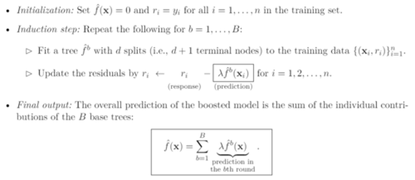
boosting algorithm

turning parameters (boosting)

1. number of trees B

2. shrinkage parameter λ

3. number of splits d

(boosting)

1. number of trees B

determines how many times we update the residuals

taking B too large may result in overfitting

it is common to select B via CV

(boosting)

2. shrinkage parameter λ aka learning rate parameter

this parameter (0<λ<1) scales down the contribution of each base tree to the overall prediction and controls the rate at which the boosting algorithm learns to prevent overfitting

(boosting)

3. number of splits d (aka interaction depth)

controls the complexity of the base trees grown

the larger the value of d, the more complex the base trees, and the higher the interaction order they accomodate

(boosting)

if λ is small, it might require

a large B to describe the residuals accurately and achieve good prediction performance

which of the following uses bootstrap samples:

bagging

random forests

boosting

bagging & random forests

which of the following samples split predictors:

bagging

random forests

boosting

random forests

for which of the following will using a large value of B generally cause overfitting:

bagging

random forests

boosting

boosting

how many turning parameters are used for each of the following:

bagging

random forests

boosting

bagging: 1

random forests: 2

boosting: 3

True/False (bagging)

the variance of the overall prediction decreases as B increases and will eventually level off

true