Simple Models: Key Vocabulary

Vocabulary flashcards covering fundamental terms and concepts from the lecture on simple models, parameter estimates, and statistical inference.

DATA = MODEL + ERROR

Fundamental statistical identity stating that each observation equals the model’s prediction plus residual error.

Observation (Y_i)

The actual recorded value for case i that we want to model or predict.

Predicted Value (Ŷ_i)

The value the model estimates for observation Y_i based on fitted parameters.

Error / Residual (e_i)

The difference between an observation and its predicted value: ei = Y_ⁱ – Ŷ_i.

Sum of Squared Errors (SSE)

The total of squared residuals; measures overall model inaccuracy and is minimized in regression.

Why Square Errors?

Squaring prevents positive and negative errors from cancelling and penalizes large misses more heavily than small ones.

• Also introduces the useful property of small penalties for very close predictions and large penalties for large misses (outliers).

Example:

• Missing by 1: 1² = 1

• Missing by 5: 5² = 25

Mean Minimizes SSE

For a single-parameter model, the arithmetic mean of Y is the value that yields the smallest possible SSE.

• It’s the best estimate until we find a useful variable.

Degrees of Freedom (df)

The number of independent pieces of information after accounting for estimated parameters; n – parameters.

• Each data point can be explained by its own unique story.

• The model tells a simple story of the data.

• Mean is an estimated parameter form our data, and uses a degree of freedom.

Baseline Model (Model C)

A model with only an intercept (mean of Y); used as a comparison standard when adding predictors.

Augmented Model (Model A)

A model that includes additional explanatory variable(s) beyond the intercept.

Parameter Count (P)

The number of estimated coefficients in a model; e.g., PA for Model A, PC for Model C.

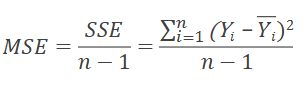
Variance (s² or MSE)

Average squared error: SSE / (n – 1); reflects typical squared miss size.

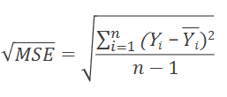
Standard Deviation (s)

Square root of variance; expresses a typical miss or data spread in original units.

• Tells us about the spread around the mean and sizes of a typical miss.

Proportion Reduction in Error (PRE)

(SSEC – SSEA) / SSEC ; proportion of error eliminated by moving from Model C to Model A.

Sum of Squares Regression (SSR)

Total variation explained by the model: Σ(Ŷ_iC – Ȳ)²; equals SSEC – SSEA for single-predictor comparison.

F-Statistic

Test ratio: [PRE / (PA–PC)] / [(1–PRE) / (n–PA)]; evaluates whether added parameter(s) significantly decrease SSE.

• A value that helps us decide if we reject the null hypothesis in regression analysis.

  • If calculated f is greater than the critical value, we reject the null hypothesis.

t-Statistic (Coefficient)

Coefficient divided by its standard error; for one predictor t² = F for overall model.

p-Value

Probability of observing a test statistic as extreme as the one obtained if the null hypothesis is true; small p suggests significance.

R-squared

Proportion of variance in Y explained by the model relative to the mean-only model (Model C).

Adjusted R-squared

R-squared adjusted for the number of predictors; penalizes unnecessary parameters.

Residual Standard Error

Square root of SSE / (n – PA); average size of prediction errors in original units.

Intercept (b0)

Estimated value of Y when all predictors equal zero; the model’s baseline level.

Slope / Coefficient (b₁)

Estimated change in Y for a one-unit change in predictor X, holding other variables constant.

Categorical Predictor Coding

Representing categories with numeric indicators (e.g., 0 = no laundry, 1 = in-unit laundry) so regression can estimate effects.

Standard Error of Coefficient

Typical distance between the estimated coefficient and its true value; smaller SE implies more precise estimate.

Confidence Interval

Range computed from estimate ± (critical value × SE) that likely contains the true parameter with a chosen confidence level.

Simple Regression

Regression with one predictor; fits a line (or two means for binary X) minimizing SSE.

Model Comparison

Evaluating whether adding predictors (Model A) improves fit over a simpler model (Model C) by testing SSE reduction.

Wordle Example

Hypothesis test comparing mean steps for common vs. uncommon words; illustrates difference-in-means via SSE framework.

Lottery Expected Value

Average payoff (probability × prize); used as comparison value in willingness-to-pay modeling example.

Error for Model C

e_i =Y_{i -} Ȳ_i.

Ȳ_i = Mean

Measures of Location (Measures of Central Tendency)

Mean, median, mode

Measures of Variability (Measures of Spread)

Standard deviation (can be squared to find variance), median absolute deviation

Model

A _______ is a way to explain variance in our DATA.

A _______ makes predictions for every observation.

Variation

_______ we have not accounted for remains in the error term.

This means, some portion of error is unexplained _______.

What is an example of a rate statistic?

Batting average in baseball is an example of a rate statistic, measuring the success of a player in hitting the ball.

What is an example of count statistics?

The number of hits, runs, or errors in a game is an example of count statistics, representing discrete outcomes.

What is Y_i?

An observed data point in row i that we want to model.

What is X_ij?

An observed data value for row i that we use to model Y_i (the value of Y_i changes as X_ij does)

What is B₁?

The “true” value for how Y_i changes as with variable(s) X_ij (that we estimate from our data).

What is b_j?

Partial regression coeffecient (partial slope) representing the weight we should give to X_ij in estimating Y_i (how much the model estimates Y_i changes with a 1 unit change in X_ij)

Regression Model

A ________ __________ minimizes SSE by fitting parameter estimates.

What is Model A’s Outcome?

b₀ + b₁X₁ + …b_j-1X_j-1 + b_jX_j + b + e_i

What is Model B’s Outcome?

b₀ + b₁X₁ + …b_j-1X_j-1 + b + e_i