Chapter 12 Descriptive stats

Frequency distributions

• Indicates the number of times each score was obtained

• X axis: score

• Y axis: # of times each score was obtained

Outliers

Scores that are unusual, unexpected, impossible, or very different from the scores of other participants

• Bar graph

• Pie chart

• Histogram (Frequency distribution): Bell-shaped curve = normal distribution)

• Frequency polygon (alt. histogram) - Study frequency of multigroups simultaneously

Two main types of descriptive stats

• Measures of central tendency

• Measures of variability

Measures of central tendency

Most important task: what is representative? What is in the middle of the data?

Mean, median, mode

Mean

X̄

Interval & ratio

Sum every score and divide by number of scores

Median

Score that divides group in half

Ordinal (Can also be used for ratio or interval)

Put all scores in order

• If odd # of scores: identify middlemost score

• If even # of scores: identify two middlemost scores, take average of them

Mode

Most frequent score

• Sometimes no mode (e.g. multiple scores have highest frequency)

• Good for all types of scales (nominal, ordinal, interval, ratio)

• Put scores in order or create a frequency distribution

• Identify the score that occurs most frequently

How do we choose which measurement of central tendency to use?

More about the mean

Since it takes into account every score, it will be affected by outliers (i.e. extreme scores)

If there are outliers, the mean might not be reflective of the “middle”

→ Outliers make more of a difference if your sample size is small

Might choose to report the median instead (or report both!!)

What are all the measures of variability

Range

Variance

Standard deviation (SD or 𝜎)

Variability

The spread of the distribution of scores

Range

To calculate: maximum score - minimum score

Variance

• Measure of the spread of a set of scores in a sample

  • ^SD²

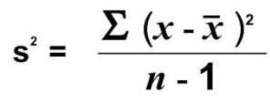
  • To calculate: sum of squared deviations around mean divided by N - 1

• The higher the variance, the greater the variability

Standard deviation

SD or 𝜎

• How far away scores tend to be from the mean on average

• Square root of the variance √s²

SD is only appropriate for ____ variables

Continuous (interval, ratio)

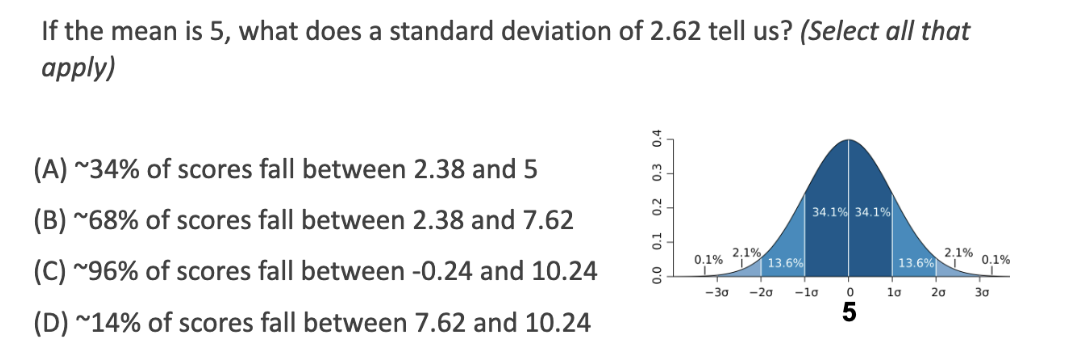
If the mean is 5, what does a SD of 2.62 tell us

So SD = 2.62

1Sigma = 5+2.62 = 7.62

-1Sigma = 5-2.62 = 2.38

And -1sigma to 1sigma falls in 68% range.

The answer is B!

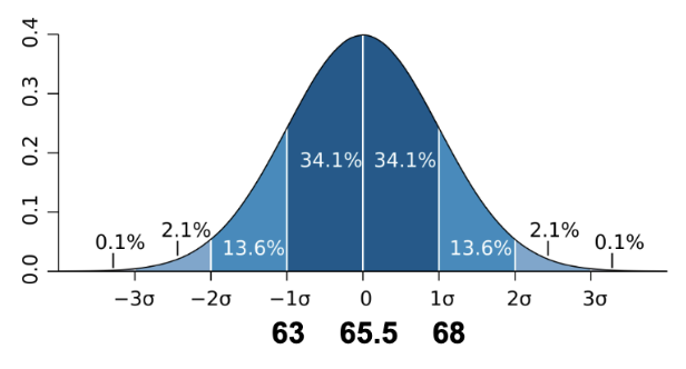
What is the SD of height

So 68 is 2.5 away from the mean (65.5), and 63 is also 2.5 away from the mean

So the SD of height is 2.5

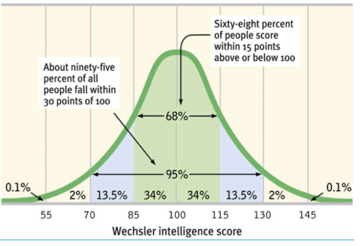
Normal distribution at what %?

In normal distribution, 68% of ppl fall in between -1SD and 1 SD, and 95% of ppl fall in between -2SD and 2SD, 99%

What measure to evaluate effect sizes between two groups?

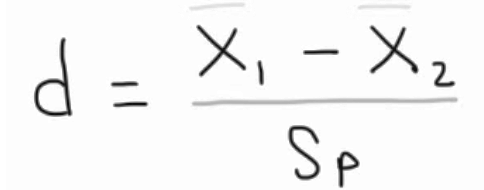
Cohen’s d

What is Cohen’s d?

Used when comparing two groups on an interval or ratio scale variable

How far apart the means are in units of SD

Cohen’s d’s formula

Xbar1 = Mean of popul.1

Xbar2 = Mean of popul.2

Sp = Standard deviation

Practice finding Cohen’s d:

Hannah uses 1-100 scale, Robert uses 1-5 scale

Hannah’s data: Sunny mean = 86, rainy mean = 70, SD = 14

Robert’s data: Sunny mean = 4.6, rainy mean = 3.5, SD = 0.7

Hannah: Mean diff is 16, SD is 14 → 16/14 =. 1.14

Robert: Mean diff is 1.1, SD is 0.7 → 1.1/0.7 = 1.57

Robert found a bigger effect size than Hannah (more, but we would not have known without Cohen’s d)

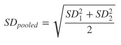
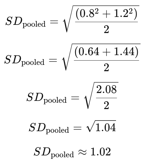
What do we do if there’s 2 SD values to calculate Cohen’s d?

Using this formula, then we can finally calculate Cohen’s d

Correlation coefficient r

• A numerical index that reflects the degree of linear relationship between two variables

• Pearson r: -1 (perfect negative) to +1 (perfect positive)

• Example: delay of gratification and academic competence (marshmallow test)

  • Variable 1: ability to delay gratification at age 5

  • Variable 2: academic competence (rated by parents) at age 15

  • Pearson r = .39

    • (0) - (.3) = small, (.3) - (.5) = medium, (.5) - (1) = large

r = .39, r² = .15

Coefficient of determination r²

Squared correlation coefficient - measure of shared variance

• how much the variables overlap. Basically correlation (r) square → coefficient of determination predicts how much of the variability in variable A predicts variability in variable B

• If r² = 0, no overlap (no shared variance)

If r² = 1, complete overlap (complete shared variance)

Answer this question

So correlation (r) is -0.36, and square of it is -0.36 x -0.36 = 0.1296

So approximately coefficient of determination (r²) is 13%

r is 0.77. Explain why B is correct

The square of the correlation coefficient, r², tells us the proportion of the variability in one variable that can be explained by the other. Here:

r² = 0.77² = 0.5929 ≈ 59%

This means that 59% of the variability in alertness can be explained by the variability in sleep duration

r² is the proportion of variance being explained

If correlation is r = .50, then r² = .25

Means that one variable accounts for 25% of the variance in other variable, and vice versa

The range of r² runs from…

0.00 (0%) to 1.00 (100%)

This r² value or squared correlation coefficient is sometimes referred to as the amount of shared variance

Ex. 0.15 = 15% shared variance = 15% of variability in v1 can be explained/predicted by v2

Consider relationship between life satisfaction and subjective health. The correlation coefficient is r = .30

Convert this to r², what did you get? Now, multiply this by 100, what does this value mean?

r² = 0.30 × 0.30 = 0.09

If we multiply this by 100, it means that 9% of the variance in life satisfaction is explained by the variance in subjective health, and vice versa

Range restriction (in correlation coefficient)

Imagine there is a moderate positive correlation between high school grades and university GPA

The whole range of highschool range is too broad on the plot graph. Just put a big circle and look at the top end (top right)

If you only look at students with the highest high school grades, it might look like there is no correlation between high school grades and university GPA

If you have a curvilinear relationship, the correlation coefficient will be….

 Zero, because correlation has to be a straight line

This doesn’t mean theree is no relationship between the variables

There may be a non-linear relationship between the variables

Regression

Uses correlation(s) between variables to make predictions 

• (Still) cannot determine causation!

• Use score on one variable (“Predictor”) to predict changes in another variable (“Criterion”)

Examples

• UBC uses your high school grades to predict your university grades

• Doctors assess your risk of heart attack based on your blood pressure

Regression models

A set of theoretically relevant predictors predicting a criterion variable

Can look at how one or more predictors can uniquely predict variability in criterion, amongst a set of predictors

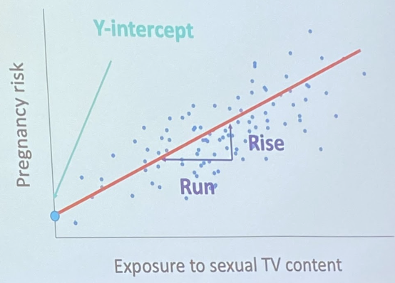
Regression line

(Similar to that basic equation y = a + bX)

Y = Criterion variable

X = predictor variable

B = slope (rise over run)

A = y-intercept

Multiple correlation

A correlation between a combined set of predictor variables and ONE criterion variable

R² (interpreted the same as r²) tells you the proportion of variability in the criterion variable that’s accounted for by the combined set of predictor variables

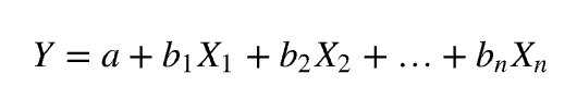
Multiple regression

More than 1 predictor (X) to predict the criterion variable

Most important benefit of repression: an investigative role of multiple predictors in independently predicting the criterion

Pregnancy and sexual TV example
To examine the contribution of each predictor..

Basically more IV (X) predicts higher DV (Y) if +bx, but more IV (X) predicts lower DV(Y) if -bx

X is the amount of predictor (hours? Days? year?)

B is slope for each correlation (Y/X)

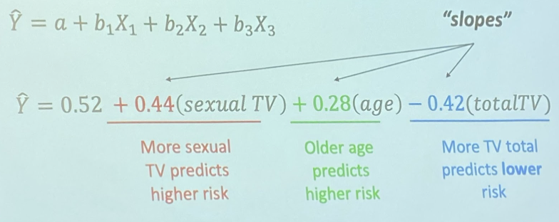
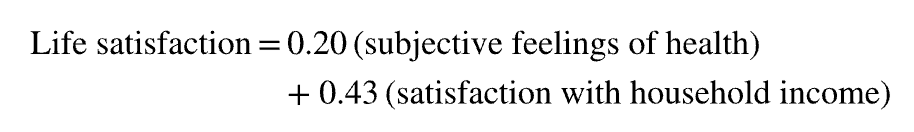
Explain this

Because the weight for income satisfaction is more than twice than for subjective health, we learn that life satisfaction has more to do with income satisfaction than feeling healthy

Partial correlation

Gives a way of statistically controlling for possible third variables in correlational analyses

It estimates what the correlation between the 2 primary variables would be if the 3rd variable were constant

To calculate, you need to have scores on the 2 primary variables of interest as well as the 3rd variable that you want to control for

Explain how this outcome of the partial correlation depends on the magnitude of the correlations between the 3rd variable and both of the two primary variables

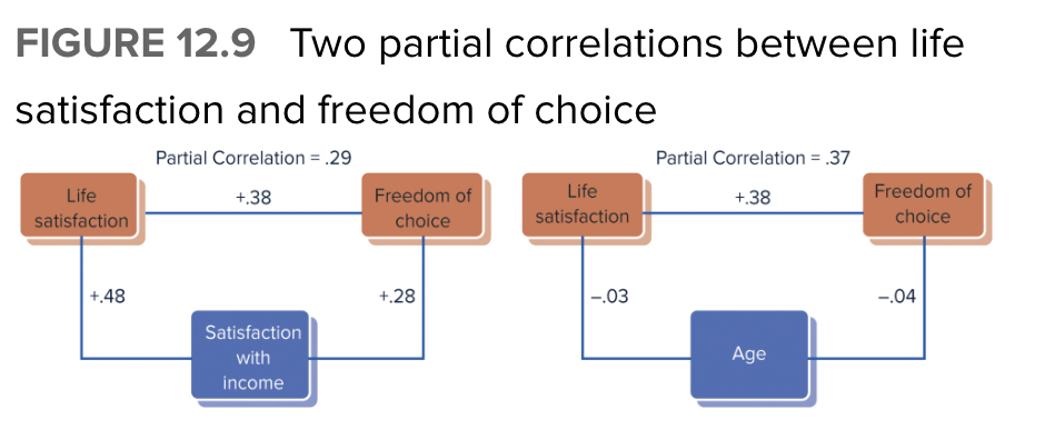
Notice that both panels show the same .38 correlation between life satisfaction and perceived freedom of choice.

Left side: The partial correlation (removing the effect of income satisfaction) drops from .38 to .29 cuz income satis. is correlated with both primary var.

Right: Age is considered as a potential third variable, however, this partial correlation remains almost the same at .37 cuz each var. is almost completely uncorrelated with age