Population Growth and Regulation

Ideal Conditions

Populations can grow rapidly

Growth Rate

In a population, the number of new individuals that are produced in a given amount of time minus the number of individuals that die

• Pop size = births – deaths (+ immigration – emigration)

Intrinsic Growth Rate (r)

The highest possible per capita growth rate for a population

• Maximum physiologically possible growth rate for a species under ideal conditions

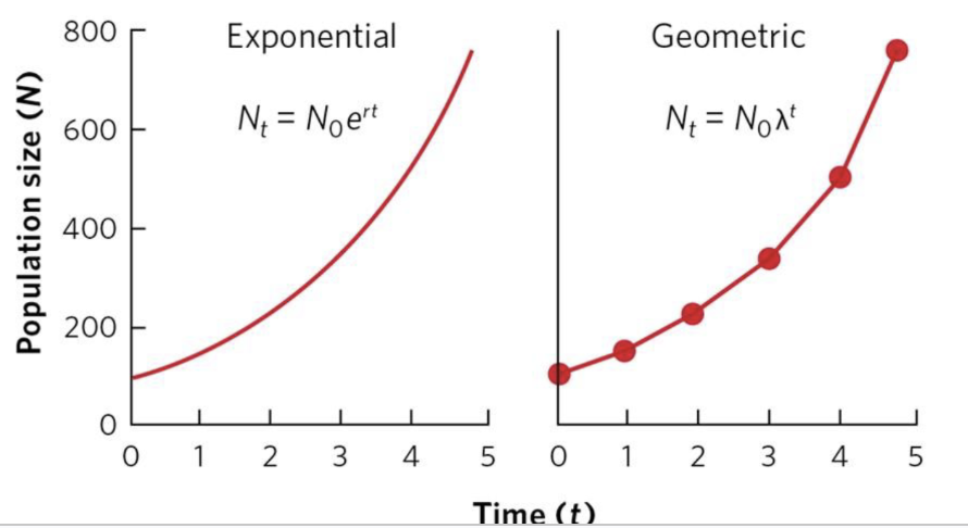
Exponential Growth Model

Model of population growth in which the population increases continuously at an exponential rate

• Assumes ideal conditions

• Assumes continuous reproduction- smoother

• N_t = N₀e^rt

  • N = population size

  • N_t = pop size at time t

  • N₀ = current pop size

  • e = constant (base of natural log)

  • r = growth rate (usually per capita)

Geometric Growth Model

Model of population growth that compares population sizes at regular time intervals

• Assumes ideal conditions

• Assumes there are reproductive seasons- bumpier

• N_t = N₀λ^t

  • N = population size

  • N_t = pop size at time t

  • λ = lambda = growth rate

    • λ = N_x / N_x-1

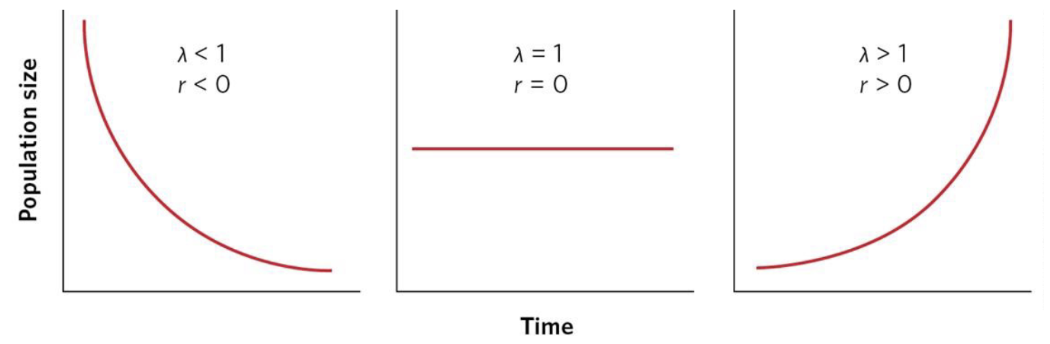
Exponential vs Geometric Growth Models

Comparison of λ and r Values when Populations are Decreasing, Constant, or Increasing

Growth Limits

Population growth is restricted by factors like limited resources, competition, and predation

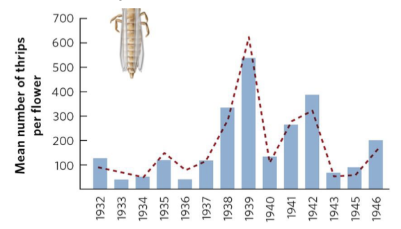
Density Independent

Factors limiting population size regardless of the population’s density

• Ex. Weather, natural disaster

• Ex. Apple Thrips (red line = estimate- models change well)

Density Dependent

Factors that affect population size in relation to the population’s density

Negative Density Dependence

When the rate of population growth decreases as population density increases

• Ex. Transmissible disease, parasites, competition

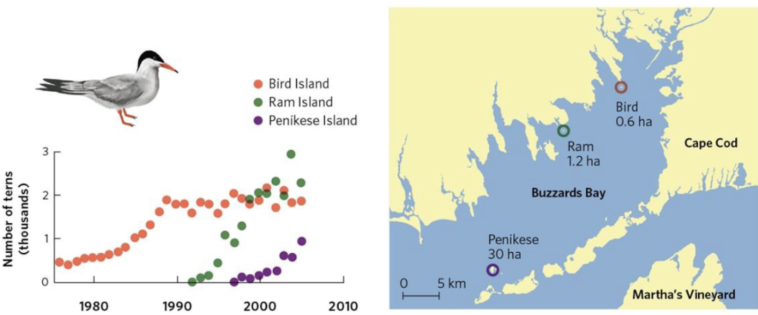
• Ex. Sea Birds

  • Live on islands

  • Growth starts exponentially → levels out → too many birds on island → some leave and colonize new island → repeat

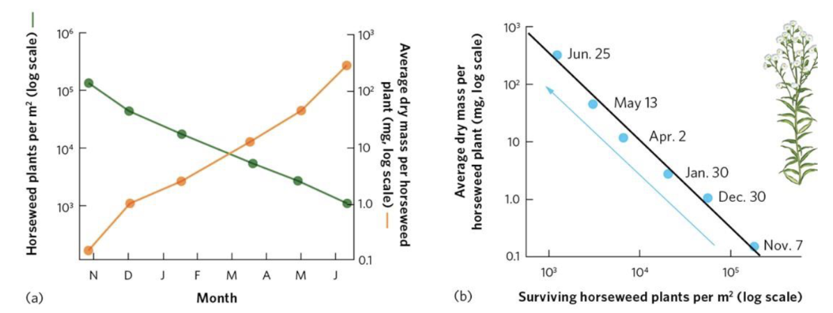
Self-Thinning Curve

Graphical relationship that shows how decreases in population density over time lead to increases in the mass of each individual in the population

• Specific example of negative density dependence

• When space becomes a limiting resource and plants start thinning

• Ex. Artificially done by farmers

  • Plant lots of seeds to account for those that don’t take → need more space → select best plants → remove others to give space to best plants

Positive Density Dependence

When the rate of population growth increases as population density increases

• Most commonly seen at the beginning of a population before resources become limited

  • More individuals = more breeding 

• Ex. Cowslip Plants

  • Many plants pollinated by wind or animals can better attract these pollinators in groups

  • Dense patch of flower more likely to get pollinated than lone flower

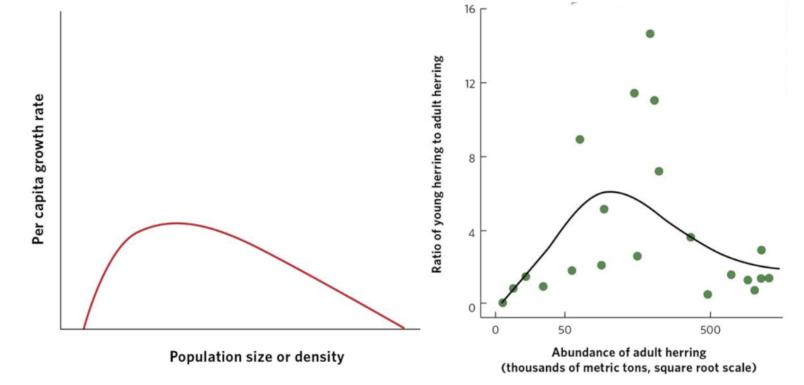
Positive and Negative Density Dependence

Most populations are governed by both

Ex. Herring (right)

• As population size increases, ratio of young to adult increases

Carrying Capacity (K)

Maximum population size that can be supported by the environment

• Can change depending on context

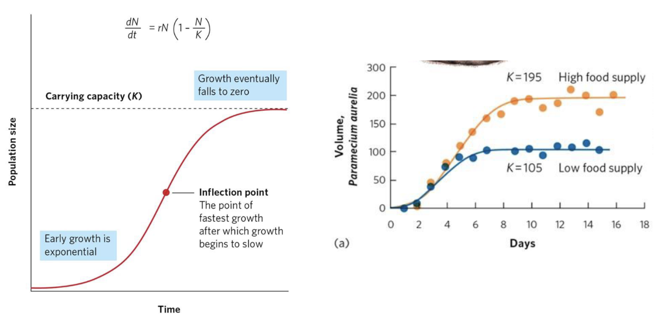
Logistic Growth Model

Growth model that describes slowing growth of populations at high densities

Inflection Point

Point of fastest growth after which growth begins to slow

• Shift from increasing growth rate to decreasing growth rate

• Point of sigmoidal growth curve at which the population achieves its highest growth rate

• Steepest slope = highest growth rate of population

Example of Logistic Growth Model

Ex. Paramecium (right)

• Manipulated amount of food available

• Showed depending on environment, carrying capacity changed

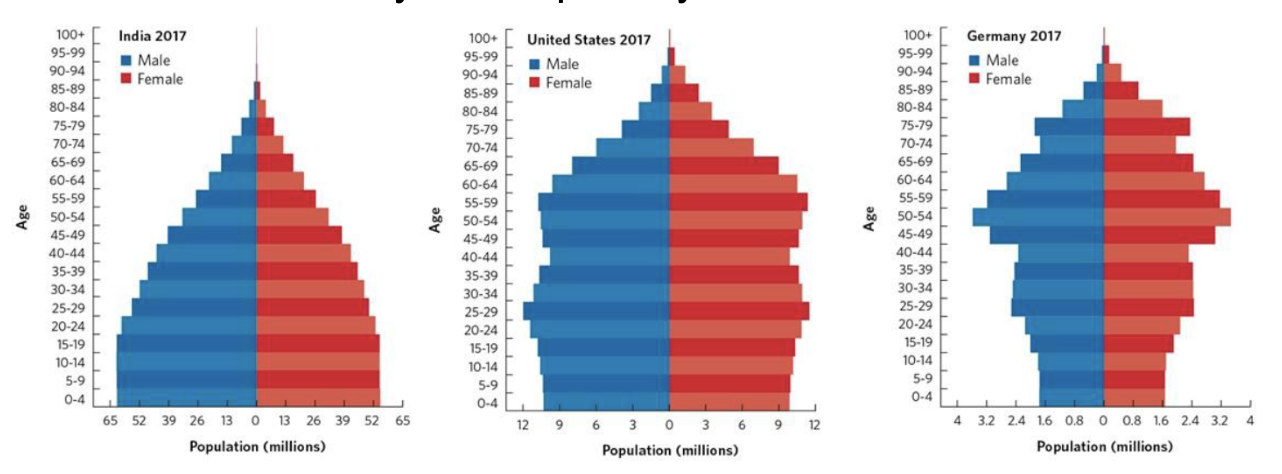
Age Structure

In a population, the proportion of individuals that occurs in different age classes

• Gives an instant picture of what a current population looks like and what the future population will look like based off shape of tables

  • Wide base = growth

  • Same width throughout = stable

  • Skinny base/top heavy = decline

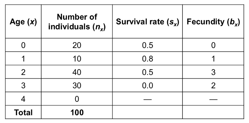
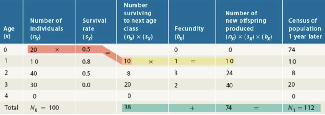
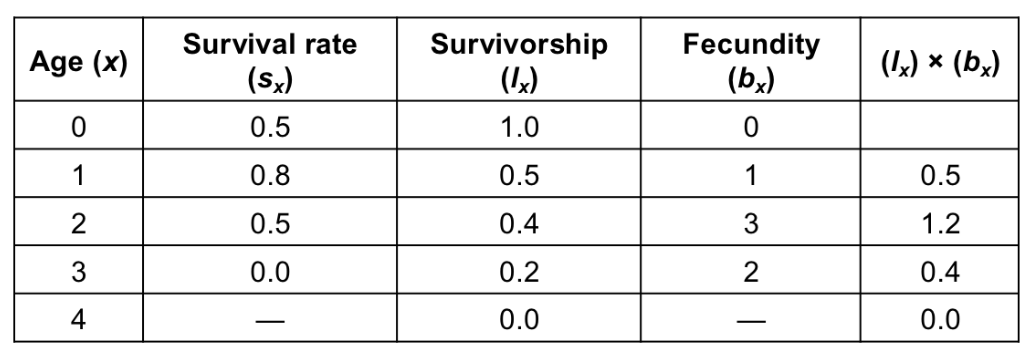
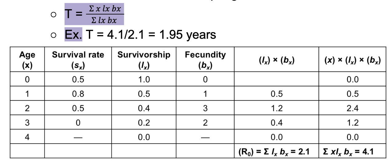
Life Tables

Tables that contain class-specific survival and fecundity (reproductive rate) data

• Demonstrate the effects of age, size, and life history stage on population growth

• Not visually friendly but allow for math

• Ex. 100 total individuals divided into 4 age classes (don’t always correspond to years, but do in this ex)

  • x = age

  • s = survival rate

  • b = fecundity

  • Read as 0 (newborns), 50% survive, none reproduce

Predictions from Life Tables

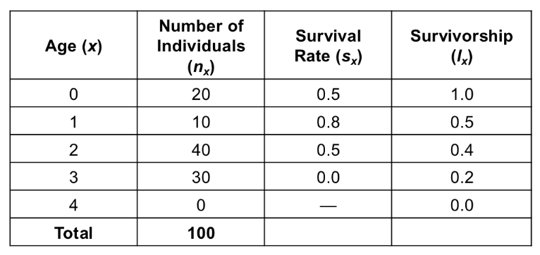
Survivorship (l_x)

Probability that an individuals survive from birth to a specified age class

• l_x = s_x-1 l_x-1

  • l = lowercase L 

• Different from survival rate

  • Survival rate is the probability of an individual to survive to next age class

  • Survivorship is probability of an individual to survive from birth to specified age class

• Survivorship for newborns is always equal to 1

  • Survivorship of newborns is the probability of newborn to survive to newborn age class (they already have)

• Ex. l₂ = (0.8)(0.5)

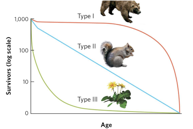
Survivorship Curves

Type 1- long lifespan

• Parental care- more likely for offspring to survive

• More k-selected species

Type 2- same probability through lifespan

Type 3- low chance of surviving until adulthood but likely to survive if they reach adulthood

• No parental care- have more babies to compensate for those that die

• More r-selected species

Net Reproductive Rate (R₀)

Total number of female offspring that we expect an average female to produce over the course of her life

• R₀ = Σ l_x b_x

• R₀ = (l₁ b₁) + (l₂ b₂) + (l₃ b₃) + …

• Expect population to be growing when R₀ greater than 2 because parents are both replaced by more offspring

• Ex. R₀ = Σ l_x b_x = 2.1

Generation Time (T)

The average time between the birth of an individual and the birth of its offspring

Cohort Life Table

Life table that follows a group of individuals born at the same time from birth to the death of the last individual

Static Life Table

Life table that quantifies the survival and fecundity of all individuals in a population during a single time interval

• Snapshot in time