BIOSCI 220 Module 1

What is the difference between R and RStudio?

What is the difference between R and RStudio?

R refers to the open source programming language used globally for a multitude of purposes.

RStudio is an interface specifically designed to facilitate communication between a programmer and their computer using R.

What are the advantages and disadvantages associated with R and RStudio being open source?

With R and RStudio being publicly accessible, users:

• have greater control and accessibility.

• can easily build upon what others have created.

• have access to a huge online support network.

Notable disadvantages include having:

• issues with software maintenance (e.g. updates).

• difficulty meeting specific requirements (e.g. having the correct drivers, device compatibility, etc.)

• vulnerability to users with malicious intent.

• difficulty overcoming the steep learning curve.

Why is the concept of reproducible research important for R and RStudio?

According to the scientific method, other people should be able to replicate your study using the same resources that you did and achieve the same result.

For R, this means that your original code/data/software/etc. should be available for and accessible to others.

What does it mean to run code?

Running code is the act of telling R to perform an action by giving it commands in the console.

What is an object?

A location where a value(s) is (are) saved.

What is a script?

A text file containing a set of commands and comments.

What are comments?

Notes written within a script to document/explain what is happening.

What is a function?

A command that performs a task in R (i.e. tells your computer what to do).

E.g. seq() generates a sequence of numbers.

What is an argument?

An input given to and used by a function to give an output.

E.g. seq(from = 8, to = 22) generates a sequence of numbers from 8 to 22.

What is a package?

A collection of specific functions, usually focused on a particular type of procedure.

What are the four basic data types in R?

Integers: whole values (eg. 0, 1, 220)
• Classified as "integer" or int

Numericals: includes integers but also fractions and decimal values (eg. -56.94, 1.3)
• Classified as "numeric" or num or dbl

Logicals: either TRUE or FALSE
• Classified as "logical" or lgl

Characters: text such as "Dog" and "Dogs are great"
• Classified as "character" or chr

How do you create an object using R?

An example of an object being created is my_pet <- "dog"
• On the left (my_pet) is the object being created, and on the right ("dog") is what we are defining it as.

Objects can be assigned a collection of things, e.g. my_pets <- c("dog" , "cat" , "bird")

What is the difference between the R functions install.packages() and library() ?

install.packages() installs a package to your computer.

library() accesses a package that has already been installed so the functions that it contains can be used.

What is a working directory in the context of R? How can this be acquired / changed?

The folder (address) where RStudio is looking for files.

• The function getwd() can be used to get the current working directory.

• The working directory can be changed by going to Session -> Set Working Directory -> Choose Directory.

How do you interpret the basic R error
## Error in library(dogtools) : there is no package called 'dogtools' ?

The package 'dogtools' may not have been installed or you may have misspelt a word(s).

How do you interpret this basic R error
## Warning in file(file, "rt"): cannot open file 'dogs.csv': No such file or directory ?

or

## Error in file(file, "rt"): cannot open the connection

You have not designated the correct location of the .csv file - there may be a typo somewhere in the location.

How do you use the appropriate R function to read in a .csv data?

An example of reading in a .csv data file would be dogs <- read_csv("C:full location of .csv").

What are some of the appropriate R functions that can be used to carry out basic exploratory data analysis with tidyverse?

• View(dogs) or glimpse(dogs) to explore the data.

• Count() function.
E.g. dogs %>%
count(Breed, Sex)

• Group_by() and summarize() functions.
E.g. dogs %>%
group_by (Fur_Colour) %>%
summarize(mean_weight = mean(Weight))

• Filter() and summarize() functions.
E.g. dogs >%>
filter(dogs, Breed == "Samoyed")
summarize(mean_weight = mean(Weight))

What is the function of the pipe operator %>% ?

%>% takes the output of one function and then "pipes" it to be the input of the next function.
• Can be read as "then" or "and then."

How do you use the the pipe operator, %>% when summarizing a data.frame?

dogs %>%
group_by(Breed) %>%
summarize(mean_weight = mean(Weight))

I.e. take the dogs data.frame then apply the group_by() function to group by Breed and then apply the summarize() function to calculate the mean weight of each group (Breed), calling the resulting number mean_weight.

How do you create simple plots of data?

Some examples:
• boxplot(Weight ~ Breed, data = dogs)
• boxplot(Age ~ Fur_Colour, data = dogs)
• boxplot(Age ~ Length, data = dogs)

• plot(Age ~ Weight, data = dogs)
• plot(dogs$Weight)

What is (indigenous) data sovereignty?

Data sovereignty is the idea that data is subject to the laws of the nation within which it is stored.

Indigenous data sovereignty perceives data as subject to the laws of the nation from which it is collected.

What is Maori data sovereignty?

Maori Data Sovereignty recognizes that Maori data should be subject to Maori governance.
• It promotes the recognition of Maori rights and interests in data and the ethical use of data to enhance Maori wellbeing.

What are the principles of Maori Data Sovereignty and how do these relate to a researcher's obligation when collecting, displaying, and analysing data?
• Whakapapa, Whanungatanga, Rangatiratanga, Kotahitanga, Manaakitanga, Kaikiakitanga.

Whakapapa (relationships): researchers must provide information about the source/purposes/context of the data's collection and the parties involved.

Whanaungatanga (obligations): researchers must ensure that the rights, risks and benefits of individuals in relation to the data match those of the groups of which they are part.

Rangatiratanga (authority): researchers must acknowledge that Maori have an inherent right to own, access, control and possess Maori data.

Kotahitanga (collective benefit): researchers must ensure that data ecosystems are designed and function in ways that enable Maori to derive a collective benefit.

Manaakitanga (reciprocity): researchers must also ensure that the collection, use and interpretation of data upholds the dignity of Maori communities, groups and individuals.

Kaitiakitanga (guardianship): researchers must ensure that Maori data is stored and transferred in a way that facilitates Maori guardianship over this data.

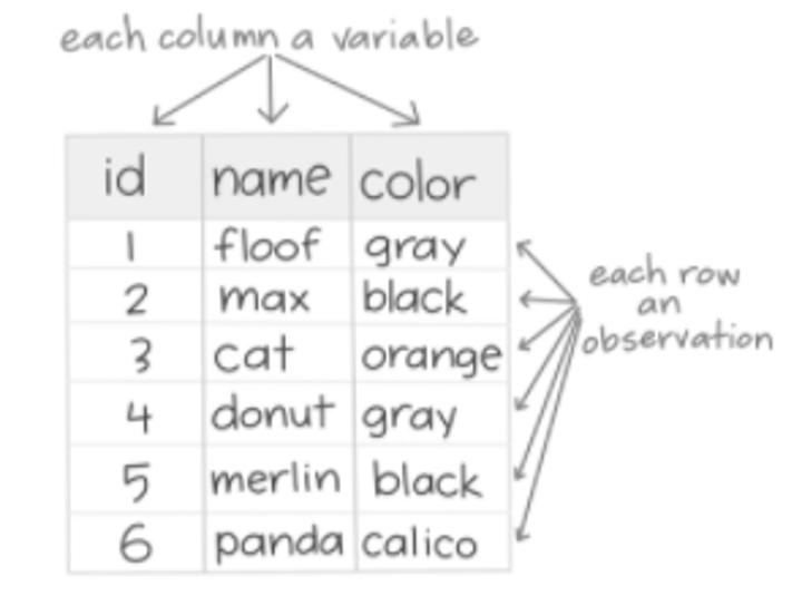
What is tidy data?

Tidy data is the required data format for performing tidyverse functions.
• Aids in reproducibility: maintains data consistency and simplicity.

1. Each variable must have its own column.

2. Each observation must have its own row.

3. Each value must have its own cell.

How could you determine the presence of NA values in your data, and how would you go about removing these values?

library(tidyverse)
dogs %>%
apply(. , 2, is.na) %>%
apply(. , 2, sum)

• Uses the is.na() function to determine if there are any NA values in the columns (represented by 2 - rows would be 1).
- Returns a TRUE if so and a FALSE if not.
• The output is then fed to the second apply() function which adds up the TRUE values.

To remove the NA values we need to create an NA free version of the data.frame.
e.g. dogs_nafree <- dogs %>% drop_na()
• This data.frame will then be used instead.

What are the features of exploratory plots?

Exploratory plots are used for exploring data, discovering new features, and formulating questions.
• Don't have to look pretty - just need to get to the point (function over form).

What are the features of explanatory plots?

Explanatory plots are designed for the audience: they have a clear purpose, are easy to read and interpret, and are not distorted.

They serve to guide the reader to a particular conclusion, answer a specific question, or support a decision (form follows function).

What are the ten simple rules for better figures?

1) Know your audience.
2) Identify your message.
3) Adapt the figure to the method of presentation.
4) Use captions.
5) Do not settle for default settings.
6) Use colour effectively.
7) Do not mislead the reader.
8) Avoid chartjunk.
9) Message trumps beauty.
10) Use the right tool (e.g. R).

What is the standard error of the mean (SEM)?

A statistical term that measures the accuracy with which a sample distribution represents a population, i.e. that reflects our uncertainty about the true population mean.

How can the standard error of the mean (SEM) be calculated in R?

The standard error of the mean is calculated by σ / √n where:
• σ is the standard deviation of the sample.
• n is the sample size.

In R, this would be done by:
sem <- dogs %>%
summarize (mean = mean(Weight), sem = sd(Weight)/sqrt(weight(Weight)))

What are the null and standard hypotheses?

According to the null hypothesis (H0), there is no difference between the characteristics of a population. Eg.
• H0: μ = 5
• H0: μHaliotis iris − μHaliotis australis = 0

However, according to the alternative hypothesis (H1), there is a difference between certain characteristics of a population. Eg.
• H1: μ ≠ 5
• H1: μHaliotis iris ≠ μHaliotis australis

What is a t-statistic and how is it calculated?

A statistic that measures the size of the difference relative to the variation in the sample data.

For a one sample t-test, t is calculated by t = x - μ / SEM where:
• x is the sample mean.
• μ is the theoretical value (proposed mean), and
• SEM is the standard error of the mean.

For an independent samples t-test, t is calculated by xdifference − 0 / SED where
• xdifference is the difference between the group averages, and
• SED is the standard deviation.

What is a p-value?

A measure of the probability under a specified statistical model of obtaining test results at least as extreme as those observed.
• i.e. the probability under the null hypothesis that we would observe a statistic at least as extreme as we did.

The smaller the p-value, the stronger the evidence against H0 (but it does NOT measure the probability that the studied hypothesis is true).

• Provides substantial evidence of a difference, NOT evidence of a substantial difference.

How can you carry out a one sample t-test in R?

t.test(paua$Length, mu = 5) where:
• mu is the true mean of the population under the null hypothesis.

This provides us with the t-statistic, degrees of freedom, p-value, alternative hypothesis, a 95% confidence interval, and the sample estimate.

How can you carry out an independent samples t-test in R?

test <- t.test(Length ~ Species, data = paua)
test (to print out the result)
test$p.value (to print out the p-value)

or

t.lm <- lm(Length ~ Species, data = paua)
summary(t.lm)$coef

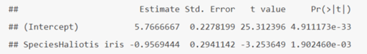
How do you interpret the output of an independent samples t-test in R (when using t.lm)?

• (Intercept) = the baseline = μHaliotis australis = 5.7666667

• SE of (Intercept) = SE of μHaliotis australis = SEM = 0.2278199

• SpeciesHaliotis iris = μHaliotis iris - μHaliotis australis = -0.9569444

• SE of SpeciesHaliotis iris = SE of (μHaliotis iris - μHaliotis australis) = SED = 0.2941142

• t value and Pr (>|t|) are the t- and p-value for testing the null hypotheses.

What is a type 1 error?

A type 1 error is when a difference is declared when there is no difference (i.e. H0 is rejected when it is actually true).

Risk is determined by the level of significance (which we set)
• α = P(Type I error) = P(false positive)

What is a type 2 error?

A type 2 error is when a difference is not declared when there is a difference (i.e. H0 not rejected when it is actually false).

Risk is determined by statistical power: the probability that the test correctly rejects the null hypothesis when the alternative hypothesis is true.
• Affected by:
- effect size (i.e. size of difference or biological significance) between the true population parameters.
- experimental error variance.
- sample size.
- type 1 error rate (α).

What is a Family-Wise Error Rate (FWER)?

The probability of making one or more type 1 errors (false positives) when performing multiple hypotheses tests.
• When making multiple comparisons, the type 1 error rate (α) should be controlled across the entire family of tests under consideration.

What are the 5 steps of performing a randomization test?

1. Decide on a metric to measure the effect in question (e.g. differences between groups means).

2. Calculate that test statistic on the observed data.

3. For a chosen number of times (nreps):
• shuffle the data labels.
• calculate and retain the t-statistics for the data.

4. Calculate the proportion of times your reshuffled statistics equal or exceed the observed.
• This is the probability of such an extreme result under the null hypothesis.

5. State the strength of evidence against the null hypothesis on the basis of this probability.

How would you perform a randomization test in R?

diff_in_means <- (paua %>% group_by(Species) %>% summarize(mean = mean(Length)) %>% summarize(diff = diff(mean)))$diff
• Creating an object for the observed difference in means.

nreps <- 1000
• Number of times you want to randomize.

randomization_difference_mean <- numeric(nreps)

for (i in 1:nreps) {
data <- data.frame(value = paua$Length)
data$random_labels <-sample(paua$Species, replace = FALSE)
• Randomise labels.
randomisation_difference_mean[i] <- (data %>% group_by(random_labels) %>% summarize(mean = mean(value)) %>% summarize(diff = diff(mean)))$diff
}
• Randomise differences in mean.

results <- data.frame(randomisation_difference_mean = randomisation_difference_mean)
• Creating an object for the results.

n_exceed <- sum(abs(results$randomisation_difference_mean) >= abs(diff_in_means))
• How many randomised differences in means are at least as extreme as the one we observed?

n_exceed

n_exceed/nreps
• Calculating the proportion.

What does a large / small p-value mean in experimental situations?

A large p-value (tail proportion) means it is likely that the randomization has produced groups differences at least as large as what we observed in our data by chance.

A small p-value means it is unlikely that the randomization has produced group differences as large as we observed in our data by chance.

What does statistical significance say about practical significance and the size of treatment differences?

Statistical significance does not imply practical significance, nor does it say anything about the size of treatment differences.

• To estimate the size of a difference you need confidence intervals.

What is a one-way ANOVA test?

A statistical procedure used to determine whether there are any statistically significant differences between the means of 3 or more independent groups.

How would you carry out a one-way ANOVA test in R?

fit.lm <- lm(bill_depth_mm ~ species, data = penguins_nafree)
anova(fit.lm)
summary(fit.lm)$coef
• Performs an F-test using anova()

or

aov <- aov(bill_depth_mm ~ species, data = penguins_nafree) summary(aov)
• Performs an F-test using aov()

What is an F-test?

A test for the existence of a difference(s) between population means.
• We test H0: all of the population means are the same, versus H1: not all of the population means are the same.

• The data gives evidence against the null hypothesis when the differences between the sample/group means is large relative to the variability within the samples or groups.

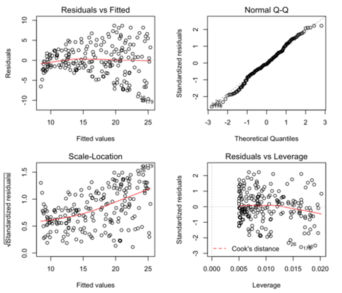
What are the key assumptions that we make when carrying out any linear regression?

What would the diagnostic plots look like if these assumptions were met?

1. Observations are independent of one another.

2. There is a linear relationship between the response and explanatory variables.
• See Residuals vs Fitted plot: horizontal line without distinct patterns = linear relationship.

3. The residuals have constant variance.
• See Scale-Location plot: horizontal line with equally spread points = constant variance.

4. The residuals are normally distributed.
• See Normal Q-Q plot: residual points following dashed line = normally distributed.

What does the equation Yi = α + β1xi + ϵi represent?

A linear regression with a simple explanatory variable, where:
• Yi is the value of the response.

• xi is the value of the explanatory variable.

• ϵi is the error term: the difference between Yi and its expected value.

• α is the intercept term (a parameter to be estimated).

• β1 is the slope: the coefficient of the explanatory variable (and a parameter to be estimated).

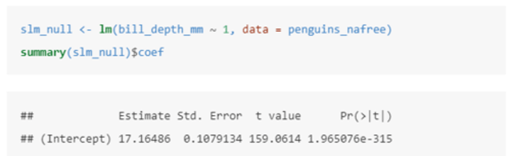
What is a one sample t-test (null / intercept only model) and how can this be carried out in R?

In this case we are testing H0: mean(average_bill_depth) = 0 vs. H1: mean(average_bill_depth) ≠ 0

This model uses the equation Yi = α + ϵi where:
• Yi is the value of the response (bill_depth_mm).
• α is the intercept (a parameter to be estimated).

In this case, the intercept tells us that the (estimated) average value of the response (bill_depth_mm) is 17.16486.

We also see that (std. error) = 0.1079134 and the t-statistic = 159.0614.

Finally, the p-value is given by Pr (>|t|) = 1.965...x10^-315

Therefore the probability of observing a t-statistic at least as extreme under the null hypothesis (average bill depth = 0) given our data is 1.965...x10^-315, giving us strong evidence against the null hypothesis.

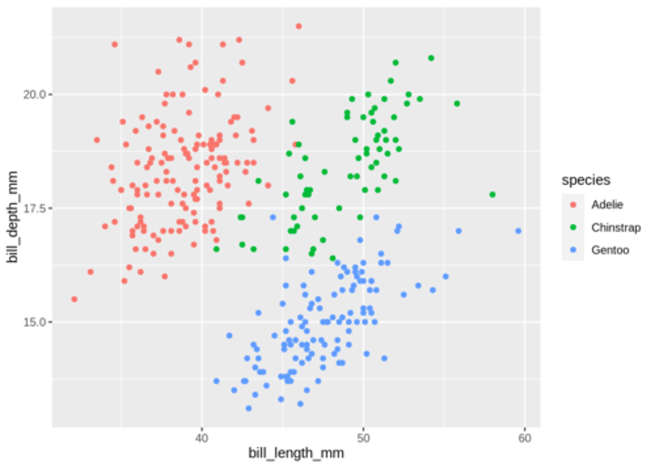
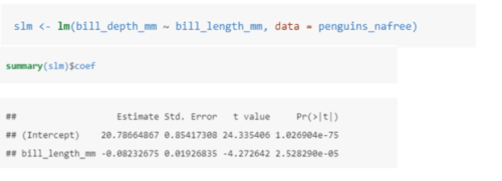
How can a variable help to explain some of the variation in another variable?

In this case we are seeing if bill_length_mm helps to explain some of the variation in bill_depth_mm.

The equation of the model is Yi = α + β1xi + ϵi where:
• Yi is the value of the response (bill_depth_mm).
• xi is the value of the explanatory variable (bill_depth_mm).
• Could also be written as bill_depth_mm = α + β1(bill_length_mm) + ϵ

In this case, the estimate (α) gives us the estimated average bill depth (mm) given the estimated relationship between bill length and bill depth.

The bill_length_mm estimate is the slope associated with bill length (mm): so for every 1mm increase in bill length we estimate a 0.082mm decrease in bill depth.

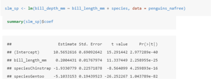
How can two explanatory variables help to explain some of the variation in another variable?

The equation of the model is Yi = β0 + β1zi + β2xi + ϵi where:
• Yi is the value of the response (bill_depth_mm).
• zi is one explanatory variable (bill_length_mm).
• xi is another explanatory variable (species).
• ϵi is the error term: the difference between Yi and its expected value.
• α, β1, and β2 are all parameters to be estimated.

In this case, the (intercept): estimate gives us the estimated average bill depth of the Adelie penguins given the other variables in the model.

The bill_length_mm: estimate (β1) is the slope associated with bill length. So for every 1mm increase in bill length we estimate a 0.2mm increase in bill depth.

The coefficients of the other species levels give the shift (up or down) of the parallel lines from the Adelie level. So given the estimated relationship between bill depth and bill length these coefficients are the estimated change from the baseline.

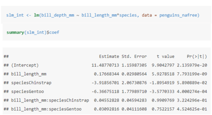
How do you include interaction effects in a model?

• An asterisk (⋆) means to include all main effects and interactions, i.e. a⋆b is the same as a + b + a:b.
- : denotes the interaction of the variable to its left and right.

In this case, the (intercept): estimate gives us the estimated average bill depth of the Adelie penguins given the other variables in the model.

The bill_length_mm: estimate (β1) is the slope associated with bill length. So for every 1mm increase in bill length we estimate a 0.177mm increase in bill depth.

The main effects of species (speciesChinstrap: estimate and speciesGentoo: estimate) give the shift (up or down) of the lines from the Adelie level - these lines are no longer parallel.
• The interaction terms (bill_length_mm: speciesChinstrap and bill_length_mm: speciesGentoo) specify the species specific slopes given the other variables in the model.

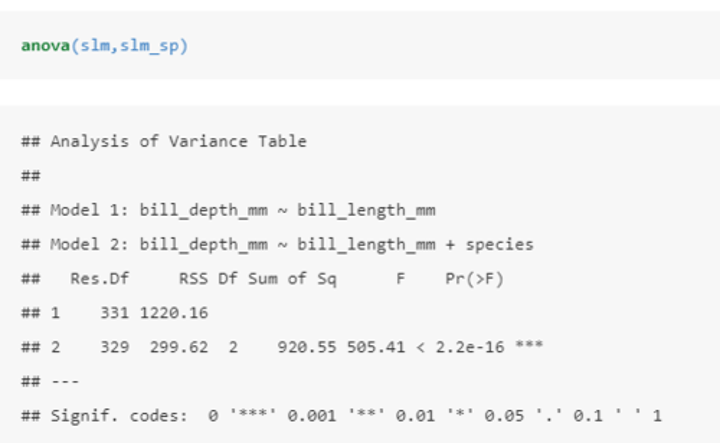
What is the purpose of nested models?

We can compare nested linear models by hypothesis testing. A nested model is a subset of another model (i.e. where some coefficients have been fixed at zero).

E.g. Yi = β0 + β1zi + ϵ is a nested version of Yi = β0 + β1zi + β2xi + ϵi where β2 has been fixed to zero.

In this case, the anova() function tests where the model (slm_sp) is just as good as capturing the variation in the data as (slm). We use the resulting p-value (2.2x10^-16 in this case) to determine if each model is as good at capturing the variation in the data (in this case we have strong evidence against this - small P value - slm_sp seems to be better at this than slm).

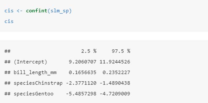
How do you produce a confidence interval for parameters of a chosen model?

In this case (for the chosen slm_sp model) the 95% confidence intervals tells us that:
• for every 1mm increase in bill length we estimate the expected bill depth increases between 0.17 and 0.24 mm.
• the expected bill depth of a Chinstrap penguin is between 1.5 and 2.4 mm shallower than the Adelie penguin.

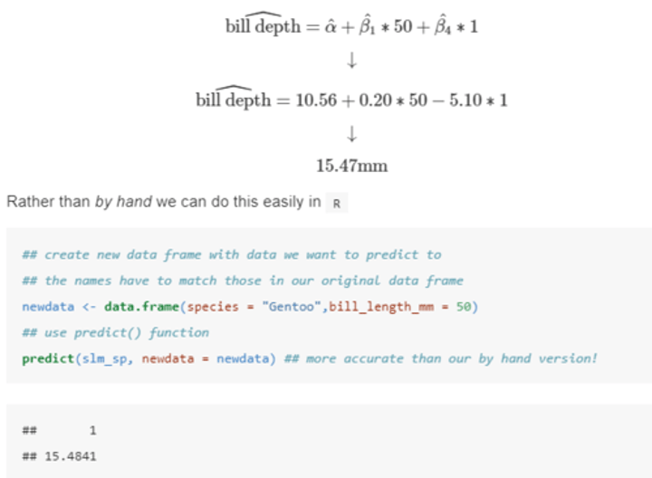
How can you perform point predictions using R?

Through the substitution of the given values into the equation.

What is an experimental unit?

The entity that we (as the researchers) want to make inferences about.
• I.e. the smallest unit of experimental material that is independently investigated.

What is a treatment?

The experimental condition that we (as the researchers) independently apply to an experimental unit.

What is an observational unit?

(Also called a statistical unit) : the entity on which a response is measured.

• If one measurement is made on each experimental unit, the observational unit is the experimental unit.
- If multiple measurements are made on each experimental unit, each unit will have >1 observational units.

Consider the biological question:
How much herbicide residue is left in a plot of sprayed soil 2 weeks post spraying?
• We compare 2 herbicides: Weedz and B180. We randomly spray each of 5 plots of weeds with Weedz and the other 5 with B180.

What is the treatment, experimental unit and observational unit for this experiment?

Treatment = herbicides (Weedz or B180).

Experimental units = plots of weeds.

Observational unit=
• plots of weeds (if a single core is taken from each plot and one measurement is taken per core).
OR
• subsample (if a single core is taken from each plot, multiple subsamples are taken from each core, and measurements are taken per subsample).
OR
• core (if multiple cores are taken from each plot and a measurement is taken from each core).

What is replication?

One of the three key principles of experimental design. The repetition of an experiment or observation under the same conditions.

What is biological replication?

When each treatment is independently applied to each of several humans/animals/plants etc.
• Used to generalize the results to a population.

What is technical replication?

When two or more samples from the same biological source are independently processed.
• Used if processing steps introduce a lot of variation.
• Increases the precision with which comparisons of relative abundances are made between treatments.

What is pseudo-replication?

When one sample from the same biological source is divided into two or more aliquots which are then independently measured.
• Used if measuring instruments produce a lot of noise.
• Increases the precision with which comparisons of relative abundances are made between treatments.

What is randomization?

One of the three key principles of experimental design.
• Ensures that each treatment has the same probability being applied to each unit and thus avoids systematic bias.
- random allocation can cancel out population bias as it ensures that any other possible causes for the experimental results are split equally between groups.

• The experiment is carried out in such a way that the variations caused by extraneous factors can all be combined under the general heading of 'chance'.

What is blocking?

One of the three key principles of experimental design whereby experimental units are divided into subsets (blocks) so that units within the same block are more similar than units from different blocks.
• Helps to control variability by making treatment groups more alike.

• Used to deal with nuisance factors: factors that have an effect on the response but are of no interest (e.g., age, class).

What is Principal Component Analysis (PCA)?

A method of feature extraction that reduces data dimensionality (number of variables) by creating new uncorrelated variables (principal components) while minimizing loss of information on the original variables.

• The first new variable (PC1) explains the most variation in the data, PC2 explains the second most, and so on.

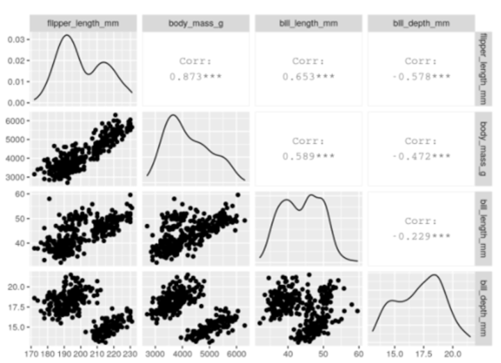
When would you carry out PCA in R?

library(GGally)
penguins_nafree %>%
select(species, where(is.numeric)) %>%
##only interested in numeric variables for PCA.
ggpairs(columns = c("flipper_length_mm", "body_mass_g", "bill_length_mm", bill_depth_mm"))

From this, we can see that a lot of these variables (e.g. flipper_length_mm, body_mass_g, bill_length_mm) are strongly (positively) related to one another.
• When combined, we could think of these three variables as telling us about the "bigness" of a penguin, thereby reducing the dimensionality of the data.

What are the three basic types of information we obtain from Principal Component Analysis (PCA)?

• PC scores: represent the coordinates of our samples on the new PC axis, i.e. the new uncorrelated variables.

• Eigenvalues: represent the variance explained by each PC which we can then use to calculate the proportion of variance in the original data explained by each axis.

• Eigenvectors (variable loadings): represent the weight that each variable has on a particular PC, i.e. the correlation between the PC and the original value.

How would you begin to carry out PCA in R?

pca <- penguins_nafree %>%
select(where(is.numeric)), -year %>%
##year makes no sense here and can be removed.
scale() %>%
##we must ensure that each variable is on the same ##scale (i.e. that changes are relative).
prcomp()
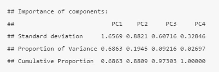
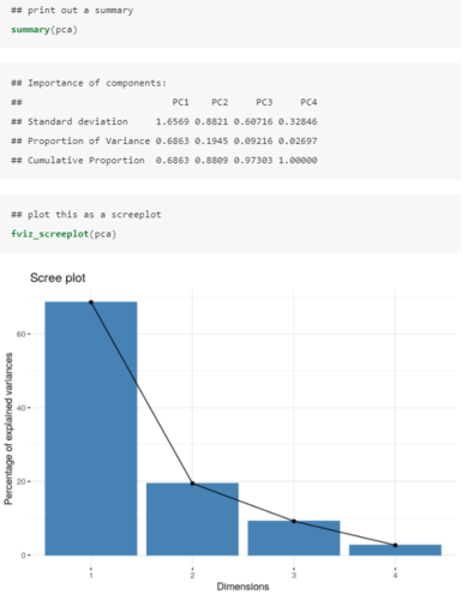
summary(pca)

The output tells us that we obtain 4 principal components (PC1-4), each of which explains a percentage of the total variation in the dataset.
• PC1 explains ~69% of the variance.
• PC2 explains ~19% of the variance.
• PC3 explains ~9% of the variance.
• PC4 explains ~3% of the variance.

From the Cumulative Proportion row we see that just by knowing the position of a sample in relation to PC1 and PC2, we can get an accurate view on where it stands in relation to other samples (as PC1 and PC2 explain a combined 88% of the total variance).

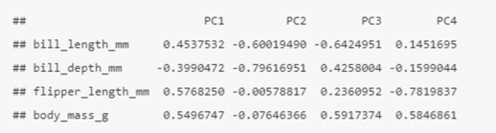
How can you see the loadings (relationship) between the initial variables and the principal components in R?

pca$rotation

Here we can see that bill_length_mm, flipper_length_mm, and body_mass_g all have strong positive relationships with PC1, whereas bill_depth_mm has a strong negative relationship with PC1.

• Relates back to the ggpairs plot, whereby bill length, flipper length and body mass (together: penguin bigness) had a strong positive relationship, while bill depth had a somewhat negative relationship with these three variables (the opposite of penguin bigness).

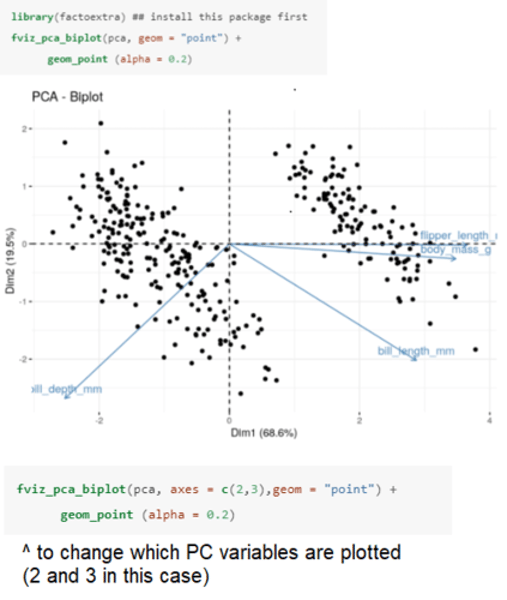
How can you illustrate the loadings (relationship) between the initial variables and the principal components in R?

Produces a biplot whereby the length of the arrows labeled by the original variables represents the magnitude of the loadings on the new variables, and where they point indicates the direction of that relationship (positive or negative).

• By default the first two new uncorrelated variables (PC1 and PC2) are plotted.

PC1 (x-axis) accounts for 68.6% of the variation.
• Bill length, flipper length, and body mass all have a strong positive relationship with PC1, while bill depth has a negative relationship with PC1.
• We can therefore think of this new variable as representing penguin "bigness".

PC2 (y-axis) accounts for just 19.5% of the variation.
• Neither flipper length nor body mass have much of a relationship with PC2 (both arrows are close to the zero line), however, both bill length and bill depth have a relatively strong negative relationship with PC2.
• Therefore we can think of this new variable as representing penguin "billness" (bill shape).

How do we determine how many PCs (new variables) we keep in R?

We want as much variance as possible explained whilst reducing the number of variables that we keep.
• PC1 (penguin "bigness") explains almost 70% of the variation in the four variables, while PCs 2, 3 and 4 explain the other 30% combined.

The rule of thumb is to look for the "elbow" in the screenplot; that is, the PC beyond which you are only explaining incrementally more variation.
• In this plot, we can see that the elbow happens at PC2.

Therefore we can simply retain PC1 (penguin "bigness") and use this new uncorrelated variable to represent the data.

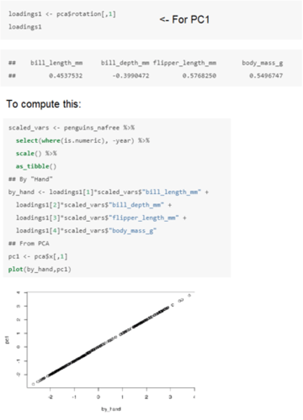
How do we obtain the principal components from the original variables in R?

The first Principal Component will be:
• 0.454 x Z1 - 0.399 x Z2 + 0.5678 x Z3 + 0.5497 x Z4

where Z1, Z2, Z3 and Z4 are the scaled numerical variables from the penguins dataset (bill length, bill depth, flipper length and body mass respectively).

What is K-means clustering?

Defining clusters (groups of data around particular values) so that the overall variation (based on the Euclidean distances between data points) within each cluster in minimized.

Identifying the optimal number of clusters (k) is important as having too many / too few can affect our ability to view overall trends.
• Too many clusters leads to overfitting (limits generalizability) while too few limits insight into the commonality of groups.

What is the procedure for K-means clustering?

1) Specify the number of clusters (k).

2) k centroids are created and are set at random as the initial cluster centres or means.

3) Each observation is assigned to its closest centroid (based on Euclidean distance).

4) The centroid of each cluster is calculated based on all observations assigned to that cluster.

5) Repeat 3) and 4) until the cluster assignments stop changing or until the maximum number of iterations is reached.

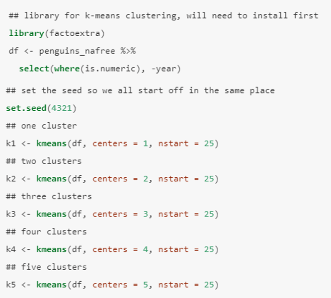
How do you perform K-means clustering in R using factoextra?

We use the kmeans() function from the factoextra package.
• The first argument of kmeans() should be the dataset you wish to cluster - df (defined as penguins_nafree) in this case.

Here we have chosen 5 clusters. Setting nstart = 25 means that R will try 25 random starting assignments and then select the best results i.e. the one with the lowest within-cluster variation.

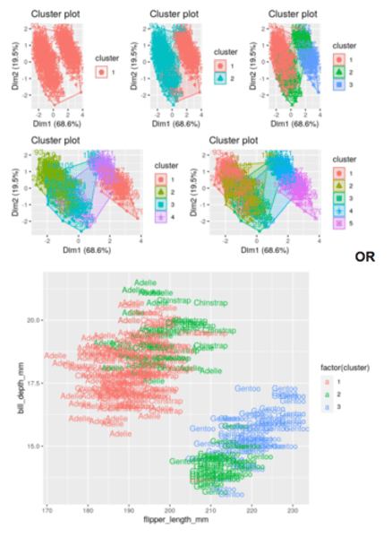
How do you determine the optimal number of clusters using the visual inspection method in R?

p1 <- fviz_cluster(k1, data = df)
p2 <- fviz_cluster(k2, data = df)
p3 <- fviz_cluster(k3, data = df)
p4 <- fviz_cluster(k4, data = df)
p5 <- fviz_cluster(k5, data = df)
library(patchwork) (p1| p2| p3)/ (p4 | p5)
##to arrange the plots

Alternatively, you can use standard pairwise scatter plots to illustrate the clusters compared to the original variables.
df %>%
mutate(cluster = k3$cluster,
species = penguins_nafree$species) %>%
ggplot(aes(flipper_length_mm, bill_depth_mm, color = factor(cluster), label = species)) + geom_text()

This is purely a visual observation.

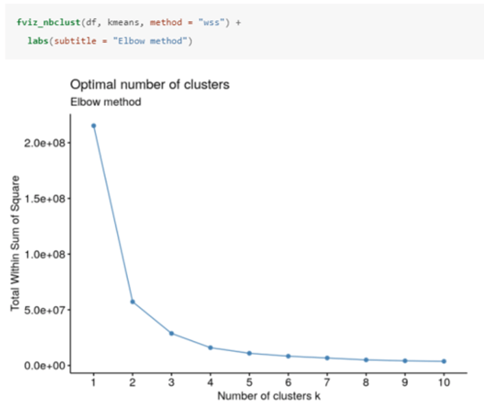
How do you determine the optimal number of clusters using the elbow method in R?

The optimal number of clusters occurs at the point in which the knee "bends", i.e. when the marginal total sum of squares begins to decrease at a linear rate.

In this case, there is an obvious bend at 2 clusters, however there is some ambiguity around 3 clusters.

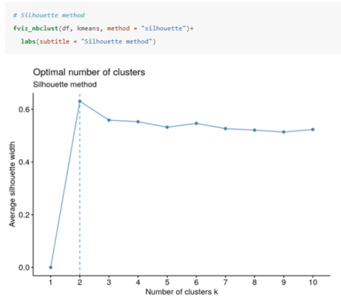
How do you determine the optimal number of clusters using the silhouette method in R?

Computes the average silhouette of observations for different values of k.

The optimal number of clusters (k) is the one that maximizes the average silhouette over a range of possible values for k (2 in this case).

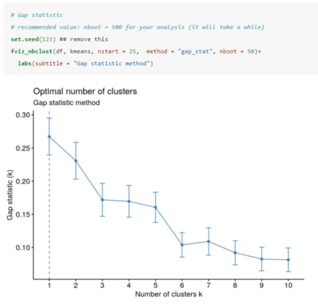
How do you determine the optimal number of clusters using the gap method in R?

The gap statistic compares the total intracluster variation for different values of k with their expected values under a null distribution (i.e. a distribution with no obvious clustering).

The optimal number of clusters (k) is the one that maximizes the gap statistic (1 in this case).

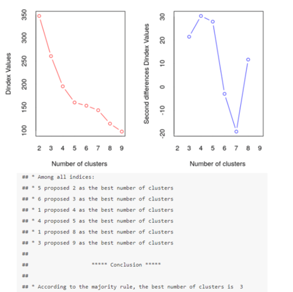
How do we make an informed decision about the optimal number of clusters?

library(NbClust)
cluster_30_indexes <- NbClust(data = df, distance = "euclidean", min.nc = 2, max.nc = 9, method = "complete", index ="all")

The Dindex is a graphical method of determining the optimal number of clusters.

In the Dindex plot produced, we are looking for a significant "knee" (a significant peak in the second differences plot) which corresponds to a significant increase in the value of the measure.

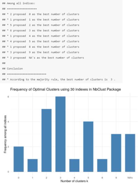
According to the majority rule, the best number of clusters is 3.

How do we make an informed decision about the optimal number of clusters? (2)

library(NbClust)
fviz_nbclust(cluster_30_indexes) + theme_minimal() + labs(title = "Frequency of Optimal Clusters using 30 indexes in NbClust Package")

Again, according to the majority rule, the best number of clusters is 3.