MM - Chapter 5: Basics of Digital Audio

what is sound?

Sound is a wave phenomenon like light, but is macroscopic and involves molecules of air being compressed and expanded under the action of some physical device

• For example, a speaker in an audio system vibrates back and forth and produces a longitudinal pressure wave that we perceive as sound.

• Since sound is a pressure wave, it takes on continuous values, as opposed to digitized ones.

Even though such pressure waves are longitudinal, they still have ordinary wave properties and behaviors, such as

• reflection (bouncing)

• refraction (change of angle when entering a medium with a different density)

• diffraction (bending around an obstacle)

If we wish to use a digital version of sound waves, we must form digitized representations of audio information

Signals can be decomposed into a sum of sinusoids. Weighted sinusoids can build up quite a complex signal.

Wat is de link tussen ‘pitch’ en ‘frequency’?

Wat zijn harmonics?

Whereas frequency is an absolute measure, pitch is generally relative — a perceptual subjective quality/property of sound

• Pitch and frequency are linked by setting the note A above middle C to exactly 440 Hz

• An octave above that note takes us to another A note. An octave corresponds to doubling the frequency. Thus, with the middle “A” on a piano (“A4” or “A440”) set to 440 Hz, the next “A” up is at 880 Hz, or one octave above

• Harmonics: any series of musical tones whose frequencies are integral multiples of the frequency of a fundamental tone

• If we allow non-integer multiples of the base frequency, we allow non-“A” notes and have a more complex resulting sound

Bespreek digitization of sound. Wat betekenen sampling en quantization?

Digitization means conversion to a stream of numbers, and preferably these numbers should be integers for efficiency

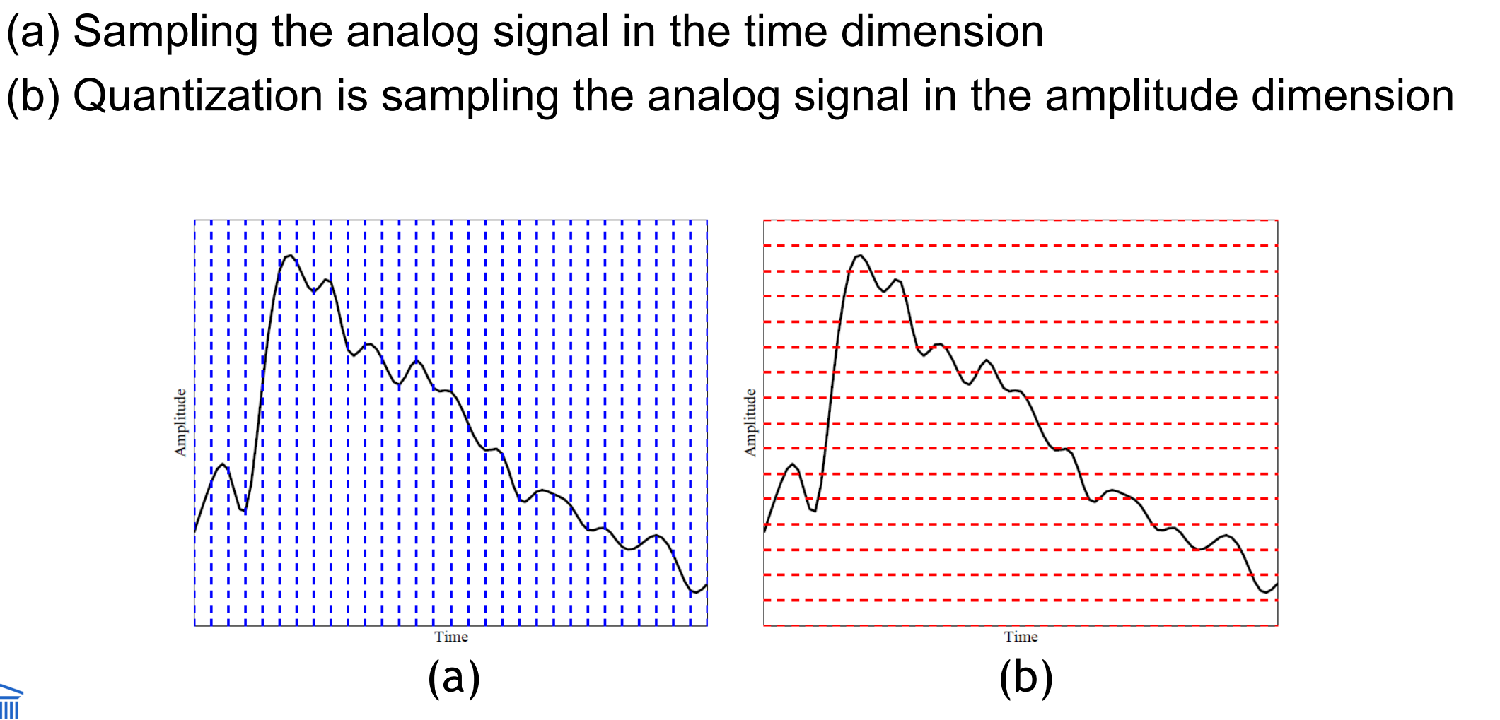
Sound has a 1-dimensional nature (amplitude depends on time)

To digitize, the signal must be sampled in each dimension: in time, and in amplitude

• Sampling means measuring the quantity we are interested in, usually at evenly-spaced intervals

• The first kind of sampling, using measurements only at evenly spaced time intervals, is simply called, sampling. The rate at which it is performed is called the sampling frequency

  • for audio, typical sampling rates are from 8 kHz (8,000 samples per second) to 48 kHz. This range is determined by the Nyquist theorem, discussed later

• Sampling in the amplitude or voltage dimension is called quantization

To decide how to digitize audio data we need to answer the following questions:

• What is the sampling rate?

• How finely is the data to be quantized, and is quantization uniform?

• How is audio data formatted and/or compressed? (file format)

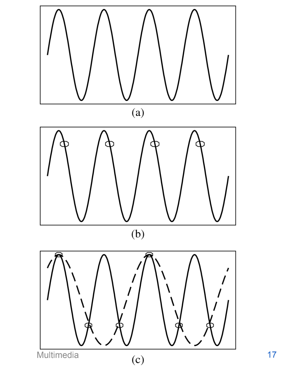
Nyquist theorem

The Nyquist theorem states how frequently we must sample in time to be able to recover the original sound

• Figure (a) shows a single sinusoid: it is a single, pure, frequency (only electronic instruments can create such ‘boring’ sounds).

• If sampling rate just equals the actual frequency, Figure (b) shows that a false signal is detected: it is simply a constant, with zero frequency.

• Now if sample at 1.5 times the actual frequency, Figure (c) shows that we obtain an incorrect (alias) frequency that is lower than the correct one — it is half the correct one (the wavelength, from peak to peak, is double that of the actual signal).

Thus for correct sampling we must use a sampling rate equal to at least twice the maximum frequency content in the signal

• This rate is called the Nyquist rate

Nyquist Theorem: If a signal is band-limited, i.e., there is a lower limit f1 and an upper limit f2 of frequency components in the signal, then the sampling rate should be at least 2(f2 − f1).

Nyquist frequency: half of the Nyquist rate

• Since it would be impossible to recover frequencies higher than Nyquist frequency in any event, most systems have an antialiasing filter that restricts the frequency content in the input to the sampler to a range at or below Nyquist frequency

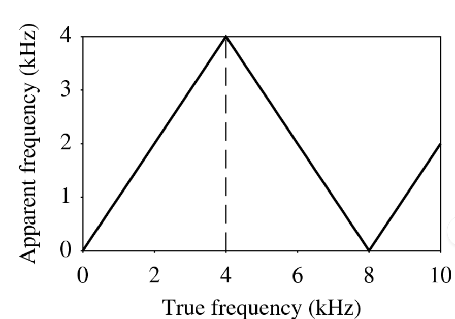
The relationship among the Sampling Frequency, True Frequency, and the Alias Frequency is as follows:
falias = fsampling − ftrue, for ftrue < fsampling < 2 × ftrue

wat is apparent frequency

In general, the apparent frequency of a sinusoid is the lowest frequency of a sinusoid that has exactly the same samples as the input sinusoid.

Figure shows the relationship of the apparent frequency to the input frequency: folding of sinusoid frequency which is sampled at 8 kHz. The folding frequency, shown dashed, is 4 kHz.

Shannon’s sampling theorem

if a signal xa(t) is bandlimited with Xa(w) = 0 for |w| > wm, then xa(t) is uniquely determined by its samples provided that ws >= 2wm. The original signal may then be completely recovered by passing xs(t) through an ideal low-pass filter.

• the frequency is ws/2 is called the Nyquist frequency

• if the condition is not satisfied, aliasing distorion occurs

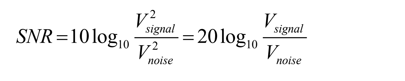
Signal to noise ratio (SNR)

The ratio of the power of the correct signal and the noise is called the signal to noise ratio (SNR) — a measure of the quality of the signal

The SNR is usually measured in decibels (dB), where 1 dB is a tenth of a bel. The SNR value, in units of dB, is defined in terms of base-10 logarithms of squared voltages, as follows:

The usual levels of sound we hear around us are described in terms of decibels, as a ratio to the quietest sound we are capable of hearing. Table shows approximate levels for these sounds.

Quantization error en Signal to quantization noise ratio (SQNR)

Aside from any noise that may have been present in the original analog signal, there is also an additional error that results from quantization.

• If voltages are actually in 0 to 1 but we have only 8 bits in which to store values, then effectively we force all continuous values of voltage into only 256 different values

• This introduces a rounding error. It is not really “noise”. Nevertheless, it is called quantization noise (or quantization error).

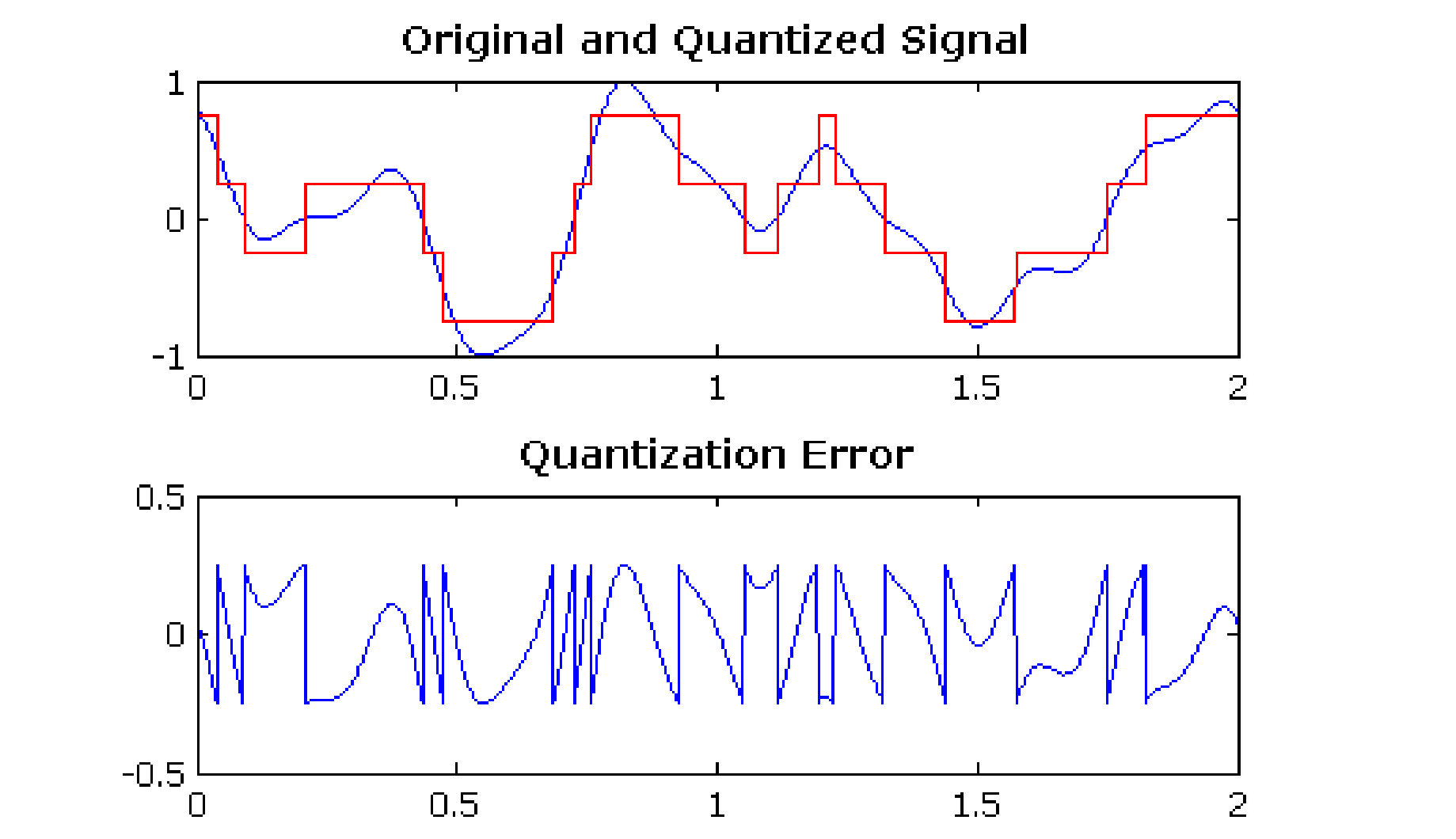
The quality of the quantization is characterized by the Signal to Quantization Noise Ratio (SQNR).

• Quantization noise: the difference between the actual value of the analog signal, for the particular sampling time, and the nearest quantization interval value.

• At most, this error can be as much as half of the interval.

linear and nonlinear quantization

Linear format: samples are typically stored as uniformly quantized values

Non-uniform quantization: set up more finely-spaced levels where humans hear with the most acuity

• Weber’s Law stated formally says that equally perceived differences have values proportional to absolute levels: ΔResponse ∝ ΔStimulus/Stimulus

Nonlinear quantization works by first transforming an analog signal from the raw s space into the theoretical r space, and then uniformly quantizing the resulting values

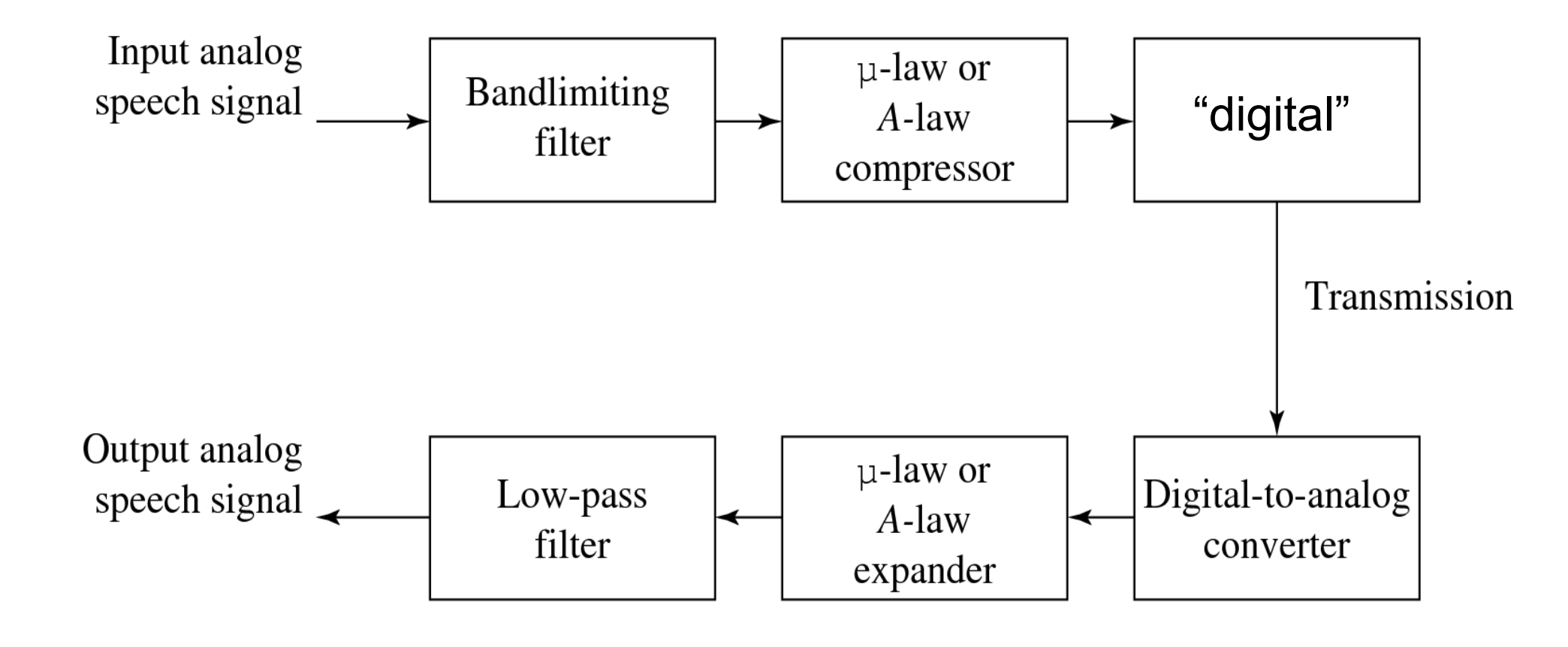
• Such a law for audio is called μ-law encoding, (or u-law). A very similar rule, called A-law, is used in telephony in Europe.

bit allocation in μ-law

In μ-law, we would like to put the available bits where the most perceptual acuity (sensitivity to small changes) is.

• Savings in bits can be gained by transmitting a smaller bit-depth for the signal

• μ-law often starts with a bit-depth of 16 bits, but transmits using 8 bits

• And then expands back to 16 bits at the receiver

audio filtering

Prior to sampling and AD conversion, the audio signal is also usually filtered to remove unwanted frequencies. The frequencies kept depend on the application:

• For speech, typically from 50Hz to 10kHz is retained, and other frequencies are blocked by the use of a band-pass filter that screens out lower and higher frequencies.

• An audio music signal will typically contain from about 20Hz up to 20kHz.

At the DA converter end, high frequencies may reappear in the output

• because of sampling and then quantization, smooth input signal is replaced by a series of step functions containing all possible frequencies.

• so at the decoder side, a low-pass filter is used after the DA circuit

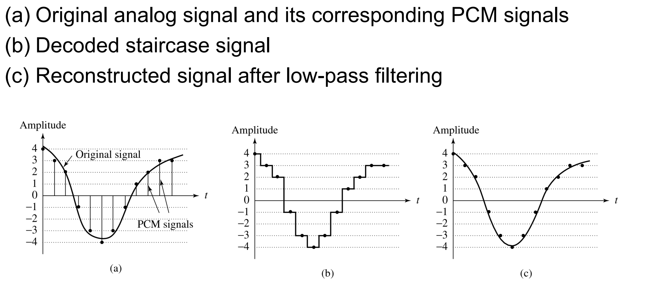
Digitization of sound volledig proces (figuur)

audio quality vs data rate (kort)

To transmit a digital audio signal, the uncompressed data rate increases as more bits are used for quantization. Stereo usually doubles the bandwidth.

Synthetics sounds (2 approaches)

FM (Frequency Modulation)

• Usually, FM is carried out using a sinusoid argument to a sinusoid

Wave Table synthesis

• A more accurate way of generating sounds from digital signals

• Also known, simply, as sampling

• In this technique, the actual digital samples of sounds from real instruments are stored

• Since wave tables are stored in memory on the sound card, they can be manipulated by software so that sounds can be combined, edited, and enhanced

Quantization and transformation of data (coding of audio)

1. stages of a compression scheme

Quantization and transformation of data are collectively known as coding

• For audio, the μ-law technique for companding audio signals is usually combined with an algorithm that exploits the temporal redundancy present in audio signals.

• Differences in signals between the present and a past time can reduce the size of signal values and also concentrate the histogram of sample values (differences, now) into a much smaller range.

• The result of reducing the variance of values is that lossless compression methods produce a bitstream with shorter bit lengths for more likely values (→ expanded discussion in Chapter 6).

Every compression scheme has three stages:

1. The input data is transformed to a new representation that is easier or more efficient to compress.

2. We may introduce loss of information. Quantization is the main lossy step ⇒ we use a limited number of reconstruction levels, fewer than in the original signal.

3. Entropy Coding. Assign a codeword (thus forming a binary bitstream) to each output level or symbol (lossless process). This could be a fixed-length code, or a variable length code such as Huffman coding (Chap. 6).

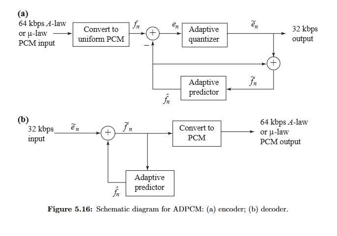
In general, producing quantized sampled output for audio is called PCM (Pulse Code Modulation).

The differences version is called LPC (for lossless) or DPCM (lossy, with quantization, and a crude but efficient variant is called DM).

The adaptive version is called ADPCM.

(herhaling datacommunicatie 😛 )

Differential coding of audio

Audio is often stored not in simple PCM but instead in a form that exploits differences — which are generally smaller numbers, so offert he possibility of using fewer bits to store.

• If a time-dependent signal has some consistency over time (“temporal redundancy”), the difference signal, subtracting the current sample from the previous one, will have a more peaked histogram, with a maximum around zero.

• For example, as an extreme case the histogram for a linear ramp signal that has constant slope is flat, whereas the histogram for the derivative of the signal (i.e., the differences, from sampling point to sampling point) consists of a spike at the slope value.

• So, if we then go on to assign bit-string codewords to differences, we can assign short codes to prevalent values and long codewords to rarely occurring ones.

Lossless predictive coding

• leg uit

• wat is het probleem + oplossing

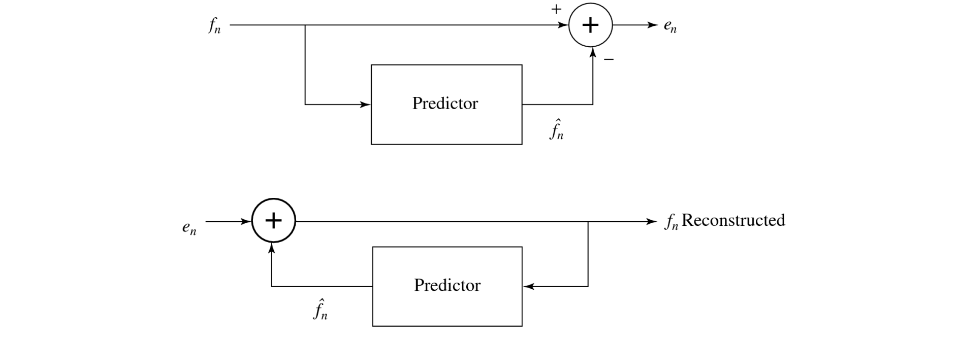
• schematic diagram (figuur!)

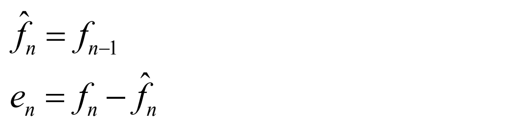
Predictive coding simply means transmitting differences — predict the next sample as being equal to the current sample; send not the sample itself but the difference between ‘previous’ and next.

• Predictive coding consists of finding differences, and transmitting these using a PCM system

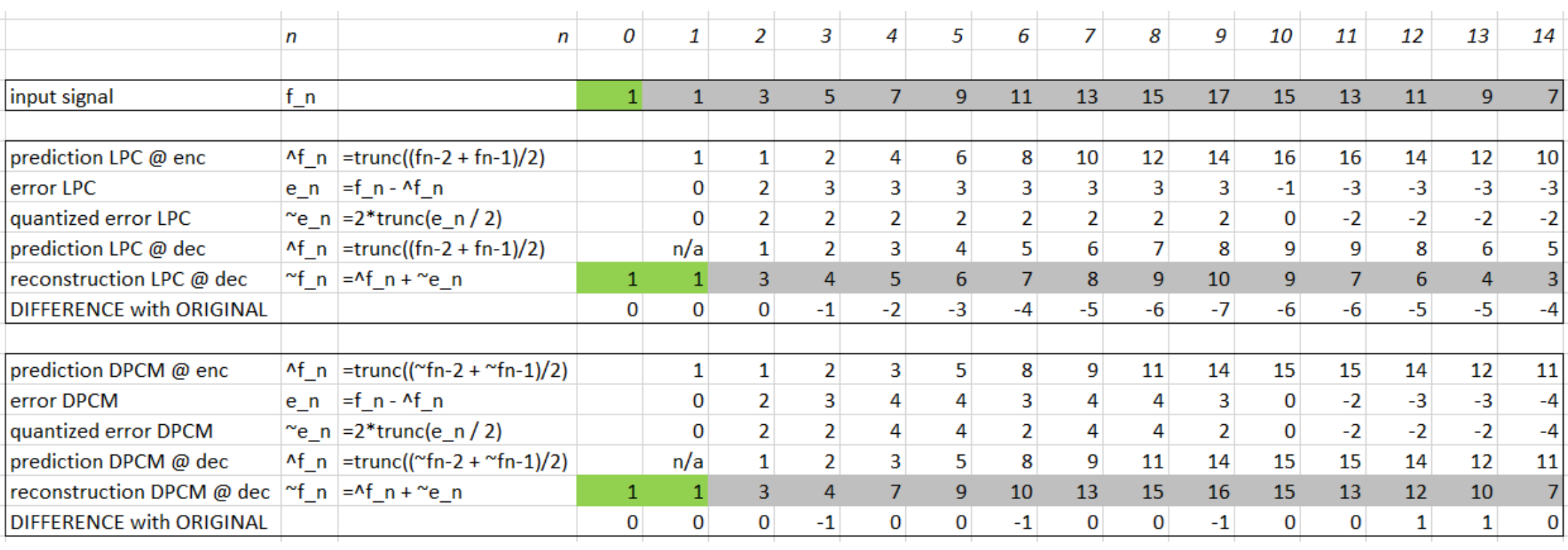
• Note that differences of integers will be integers. Denote the integer input signal as the set of values fn. Then we predict values ˆfn as simply the previous value, and define the error en as the difference between the actual and the predicted signal:
  

  

• But it is often the case that some function of a few of the previous values, fn−1, fn−2, fn−3, etc., provides a better prediction. Typically, a linear predictor function is used:

  

One problem: suppose our integer sample values are in the range [0,255]. Then differences could be as much as [-255,255] —we’ve increased our dynamic range (ratio of maximum to minimum) by a factor of two → need more bits to transmit some differences.

• A clever solution for this: define two new codes, denoted SU and SD, standing for Shift-Up and Shift-Down. Some special code values will be reserved for these.

• Then we can use codewords for only a limited set of signal differences, say only the range [-15,16]. Differences which lie in the limited range can be coded as is, but with the extra two values for SU, SD, a value outside the range [-15,16] can be transmitted as a series of shifts, followed by a value that is indeed inside the range [-15,16].

• For example, 100 is transmitted as: SU, SU, SU, 4, where (the codes for) SU and for 4 are what are transmitted (or stored).

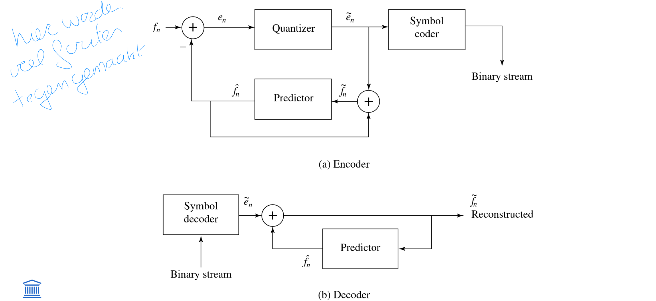
Differential Pulse code modulation (DPCM)

• wat

• stappen

• schematic diagram (figuur!)

Differential PCM is exactly the same as Lossless Predictive Coding, except that it incorporates a quantizer step.

• One scheme for analytically determining the best set of quantizer steps, for a non-uniform quantizer, is the Lloyd-Max quantizer, which is based on a least-squares minimization of the error term.

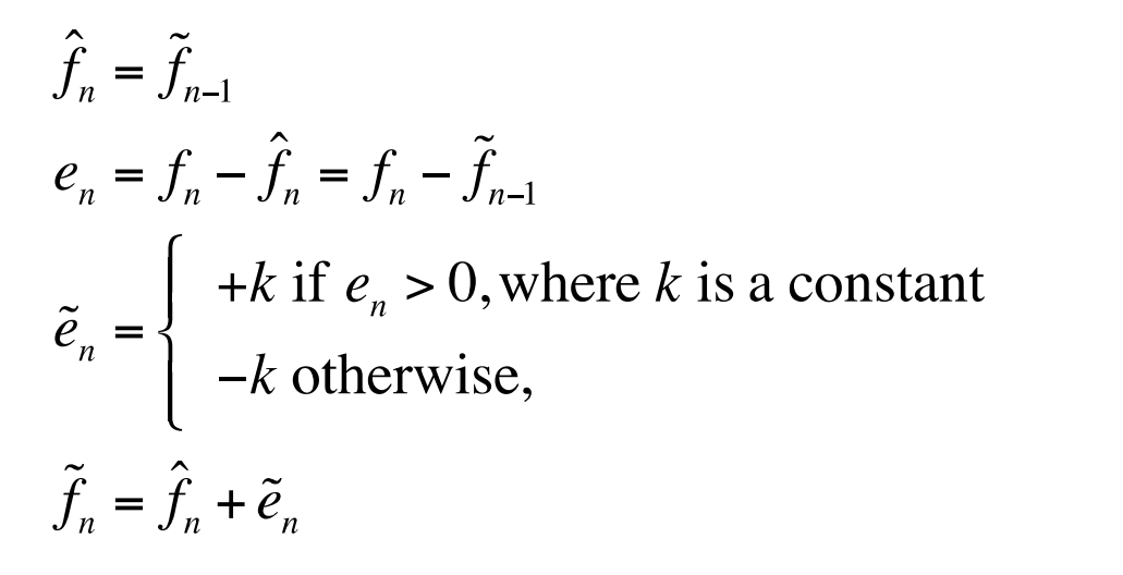
• Nomenclature:

  • signal values fn: the original signal

  • ^fn : the predicted signal

  • ~fn : the quantized, reconstructed signal

Steps in a DPCM encoder:

1. form the prediction

2. form error en by subtracting the prediction from the actual signal

3. quantize the error to a quantized version ~en

4. assign codewords for quantized error values ~en using entropy coding, e.g. Huffman coding (Chapter 6)

The distortion is the average squared error ( en - ~en = fn - ~fn)

One often plots distortion versus the number of bit levels used. A Lloyd-Max quantizer will do better (have less distortion) than a uniform quantizer

Belang van feedback loop bij dpcm

als je quantization toepast op e_n in normal forward LPC veroorzaak je drift

(drift = niet in sync zijn van encoder en decoder)

Delta modulation

• uniform delta DM

• adaptive DM

Simplified version of DPCM, often used as a quick AD converter

Uniform-Delta DM: use only a single quantized error value, either positive or negative (1-bit coder)

• produces coded output that follows the original signal in a staircase fashion.

• the prediction simply involves a delay.

• the set of equations is:

  

However, DM copes less well with rapidly changing signals. One approach to mitigating this problem is to simply increase the sampling, perhaps to many times the Nyquist rate.

Adaptive DM
If the slope of the actual signal curve is high, the staircase approximation cannot keep up. For a steep curve, one could/should change the step size k adaptively

Adaptive DPCM

ADPCM (Adaptive DPCM) takes the idea of adapting the coder to suit the input much farther. The two pieces that make up a DPCM coder: the quantizer and the predictor.

For the quantizer, we can change the step size as well as decision boundaries, using a non-uniform quantizer.

• Forward adaptive quantization: use the properties of the input signal

• Backward adaptive quantization: use the properties of the quantized output (in the encoder). If quantized errors become too large, we should change the non-uniform quantizer.

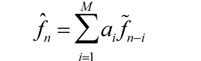
We can also adapt the predictor by adaptively changing the predictor coefficients

• using forward or backward adaptation.

• sometimes called Adaptive Predictive Coding (APC)

  • recall that the predictor is usually taken to be a linear function of previous reconstructed quantized values, ~fn​

  • The number of previous values used is called the “order” of the predictor. For example, if we use M previous values, we need M coefficients ai​, i = 1...M in a predictor:

    

However we can get into a difficult situation if we try to change the prediction coefficients, that multiply previous quantized values, because that makes a complicated set of equations to solve for these coefficients:

• Suppose we decide to use a least-squares approach to solving a minimization trying to find the best values of the ai​:

  

• Here we would sum over a large number of samples fn​, for the current patch of speech. But because ^fn​ depends on the quantization we have a difficult problem to solve. As well, we should really be changing the fineness of the quantization at the same time, to suit the signal’s changing nature; this makes things problematical.

• Instead, one usually resorts to solving the simpler problem that results from using not ~fn​ in the prediction, but instead simply the signal fn​ itself. Explicitly writing in terms of the coefficients ai​, we wish to solve:

  

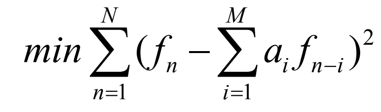
• Differentiation with respect to each of the ai​, and setting to zero, produces a linear system of M equations that is easy to solve.(The set of equations is called the Wiener-Hopf equations.)

figuur adpcm