AP PRECALC

terms and formulas

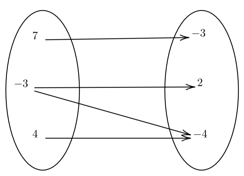
Relations

• 2 different quantities and how they relate to one another

• represented by a diagram, equation, or list

• can be written out in ordered pairs for diagram

  • not all elements have to be used

  • some inputs have multiple outputs which makes it NOT a function

relation ≠ function; function = relation

function

relation that maps a set of input values to set of output values

• can be represented verbally, numerically, algebraically, and graphically

• variable representing INPUT values: INDEPENDENT

• Variable representing OUTPUT values: DEPENDENT

function = relation; relation ≠ function

Domain

largest possible set of numbers that can be an input (x) for which the output (f(x)) is a real number

• x-axis

• furthest left= lower bound

• furthest right= upper bound

range

set of all values y can have as x takes on each its values

filled dot vs hollow dot

Filled dot → includes value in the domain or range

Hollow dot -→ does not include value

inflection points

• NOT the same thing as turning points

• it is where concavity changes from up to down or vise versa

turning points

• where the value of the change of the function changes sign- increasing to decreasing or vice versa

• occurs at the minimum or maximum (ex: vertex of parabola)

interval notation- using [-,-] and (-,-)

[-,-] includes value(s)

(-,-) does not include value(s)

use U in between for ‘union’

Domain restrictions

1. Denominator≠0

2. Can’t take square root of negative number

X and Y intercepts

X-intercept: when f(x)= 0

• zeros, solution

Y-intercept: when x=0

A function can have more than 1 x-intercept but can only have 1 y-intercept

Average rate of change

change in one value of one quantity divided by change in value of another quantity

• average speed= change in distance/change in time

• slope= deltay/deltax=(y₂-y₁)/(x₂-x₁)

• It is impossible to find average rate of change given one point but to approximate, choose points close to that given point to calculate slope with given slope to create secant line to approach similar value

slope- intercept form

y=mx+b

point-slope formula

y₂-y₁=m(x₂-x₁)

standard form of quadratic function (parabola)

ax² + bx + c = 0

Rate of Change of Quadratic Funtion

• determine average rate of change by finding slope of segment that connects to 2 points on parabola (finding slope of secant)

Polynomial functions

• always written in descending order

• if exponents are NOT a whole number→ it is NOT a polynomial function

Number of solutions/zeros/x intercepts of a function (real and non real)
= Degree of function

= Degree of function

Sine/ Sin

Opposite / hypotenuse

Cosine/Cos

Adjacent / Hypotenuse

Tangent/ Tan

Opposite / Adjacent

Y/x

sin/cos

Csc- cosecant

Reciprocal of sin

Hyp. / opposite

1/sin

Sec- secant

Reciprocal of cos

Hyp. / adjacent

1/cos

Cot- cotangent

Reciprocal of tangent

Cos/sin

x/y

Vertical translation

F(x)—> f(x) +d

(x,y)—> (x+c,y)

Up (positive) or down (negative)

Horizontal Translation

F(x) -> f(x-c)

(x,y) -> (x-c,y)

Right (negative) or left (positive)

Vertical Stretch/ Compression (Dialation)

F(x) —> af(x)

(x,y)—>(x,ay)

If a> 1 : stretch

If 0>a>1 : compression

Reflection over x-axis

F(x) —> -f(x)

(x,y) → (x,-y)

Reflection over y axis

F(x) —> f(-x)
(x,y) → (-x,y)

Horizontal stretch/ compression/ dialation

f(x)—> f(kx)

(x/k,y)

k>1 compression

0<k<1 stretch

Composite Funtion

A function that is made up of combination of transformations

y=af(b(x+c))+d

a- vertical stretch/compression

b- horizontal stretch/compression

c- horizontal shift

d- vertical shift

Imaginary number-i

powers of i

i=√-1

i²=-1

i³=i²(i)=-i

i⁴=i²(i²)= -1(-1)=1

powers continue following pattern

adding with i

add coefficients

2i+3i=5i

subtracting with i

subtract coefficients

7i-3i=4i

multiplication with i

multiply coefficients, add exponents

2i(5i)=10i²

division with i

exponents are subtracted

coefficients are divided

49i⁵/7i³= 7i²=-7

negative exponent

take reciprocal

ex. 2^-2=1/2²=1/4

fractional exponent

take root

ex. 8^2/3=³√8²= ³√64=4

x^m(xⁿ)

x^m+n

Sum of exponents

(x^m)ⁿ

x^m(n)
Product of exponents

rational exponent law: a^x/y

=^y√(a^x) =(^y√a)^x

45 45 90 triangle

side 1- a

side 2- a

hypotenuse-√2

30 60 90 triangle

side 1- a

side 2- a√3

hypotenuse- 2a

law of sines

side of triangle ABC/sine of angle opposite side

= a/sinA

=b/sinB

=c/sinC

law of cosines

a² = b² + c² - 2bc cosA

b² = a² + c² - 2ac cosB

c² = a² + b² - 2ab cosC

Function tests

Vertical line test- Is it a function

Horizontal line test- Is it one to one?

• if not, the function does not have an inverse

Extreme Value Theorem

If a polynomial function f is on a closed interval [a,b] then f has both a minimum and maximum value on [a,b]

Local extrema theorem

A polynomial function of degree n has at most n-1 realtive maxima/minima

• ex. ±x²→has one (2-1) max/min.

Absolute extrema

can occur at either relative extrema or at endpoints of CLOSED interval

Zeros (real and complex)

• on x-axis

• when equation is set to 0 (when y=0)

• polynomial function of degree n will have exactly n total zeros (real and nonreal)

Quadratic real roots

if discriminant ( -b²-4ac) is…

• >0 → 2 real roots

• =0 →1 real root

• <0→no real roots

nonreal zero of polynomial

If a+bi is a nonreal zero of a polynomial p. its conjugate a-bi is also a zero of p

even function

if equation remains unchanged when x is replaced with negative x

• f(-x)=f(x) for all x

• symmetrical to y axis

odd function

if replacing x with -x changed sign of each term of the equation to its opposite

• when f(-x)=-f(x)

End behavior of all polynomial functions

positive leading coefficient & even degree:

limx→∞p(x) =∞

limx→−∞p(x) =∞

positive leading coefficient & odd degree:

limx→∞p(x) =∞

limx→−∞p(x) =−∞

negative leading coefficient & even degree:

limx→∞p(x) =−∞

limx→−∞p(x) =−∞

negative leading coefficient & odd degree:

limx→∞p(x) =−∞

limx→−∞p(x) =∞

Positive leading coefficient & even degree end behavior:

limx→∞p(x) =∞

limx-→−∞p(x) =∞

positive leading coefficient & odd degree end behavior:

limx→∞p(x) =∞

limx→−∞p(x) =−∞

negative leading coefficient & even degree end behavior:

limx→∞p(x) =−∞

limx→−∞p(x) =−∞

negative leading coefficient & odd degree end behavior:

limx→∞p(x) =−∞

limx→−∞p(x) =∞

rational function

represented as quotient of 2 polynomial functions

• ex. h(x)=f(x)/(g(x)

• may be discontinuous (have breaks in the graph)-→ asymptotes and holes

can model data sets/scenarios including quantities that are inversely proportional

vertical asymptote

• when a rational function is undefined from an x value

• when an x value makes the denominator= 0 (cannot divide by 0)

horizontal asymptote (end behavior asymptote) rules

• if numerator degree< denominator degree, y=0

• if numerator degree = denominator degree, y = leading coefficient ratio

• if numerator degree> denominator degree by exactly 1, slant/oblique asymptote

• if numerator degree > denominator degree by MORE than 1, no horizontal asymptote

*IT IS POSSIBLE FOR A GRAPH OF RATIONAL FUNCTION TO INTERSECT A HORIZONTAL ASYMPTOTE OR SLANT ASYMPTOTE BUT IT WILL NEVER CROSS VERTICAL ASYMPTOTE*

linear parent function

f(x)=x

• Domain and Range set of real numbers

• odd function→ has origin symmetry

• includes point (0,0)

• increases throughout domain

Models data sets/scenarios that demonstrate constant rates of change

Quadratic parent function

f(x)=x²

• Domain and Range set of real numbers

• even function→ has y-axis symmetry

• includes point (0,0)

• decreases then increases

• has relative extrema

model data sets/scenarios that demonstrate linear rates of change (ex. area or 2D)

Cubic function parent function

f(x)=x³

• Domain and range is set of real numbers

• odd function→ has origin symmetry

• includes point (0,0)

• increases throughout domain

Model geometric contexts involving volume or 3D

square root parent function

f(x)=√x

• domain and range is set of all positive real numbers

• neither negative or even fuction

• includes point (0,0)

• increases throughout its domain.

reciprocal parent function

f(x)= 1/x

• Domain and range is all real numbers except 0;

• Odd function→origin symmetry

• x-axis and y-axis are asymptotes

  • decreases on intervals (-∞, 0) and (0,∞)

absolute value parent function

f(x)=|x|

• Domain is set of real numbers

• odd function→ has origin symmetry

• includes point (0,0)

• decreases then increases

sine function- even or odd?

odd function

symmetrical about the origin

cosine function- even or odd?

even function

symmetrical about the y-axis

identity function

the composition of a function f and its inverse function f-1 is the identity function

f(f^-1(x))=f^-1((f(x))

composite function

• functions linked to form new function by using output of one function as the input in other function as the input to the other function

Inverse functions

• given function f(x), if f(a)=b, then f^-1(b)=a

  • if function consists of input-output pairs (a,b) the inverse function consists of input-output pairs (b,a)

  • one-to-one check→ using horizontal line test; if any 2 different inputs in domain correspond to two different outputs in range then it is one-to-one

    • not one-to-one if two different inputs correspond to the same output, it does not have an inverse

• algebraically solving inverse functions- swap x and y values

inverse of each other test

if f(g(x))=x and g(f(x))=x then they are inverses of each other

exponential functions

• general form- f(x)= ab^x

  • where a= initial value; a≠0

  • b=base; b>0, b≠0; also the growth factor/rate

• domain is all real numbers, range is (0,-∞)

• y-intercept is (0,1)

• horizontal asymptote at y=0

• when a>0 and b>1→ exponential growth

• when a>0 and 0>b>1→ exponential decay

• does not have extrema unless on closed interval

• when a>0 and b>0→ concave up

• when a<0 and b<1→ concave down

• does not have inflection points

• end behavior possibilities:

  • lim x→± ∞ f(x)= ∞

  • lim x→ ± ∞ f(x)= -∞

  • lim x→ ± ∞ f(x)= 0

Exponential growth

• when a>0 and b>1

• when given a rate in % for word problems, add one to growth factor (decimal form)

  • ex a(1+r)^x

Exponential decay

• when a>0 and 0>b>1

  • when given a rate in % for word problems, subtract growth factor from one

    • ex a(1-r)^x

sequence vs. series

sequence= a list of numbers in a specific order

series= the sum of the terms of a sequence.

Residuals

observed value- predicted value from regression equation

residual plot: graph that shows residuals on vertical axis and the independent variable on horizontal axis

• if there is a pattern, then that regression models the data; if it is random then it doesn’t

Arithmetic sequence

• linear

• a_n=a₁+ (n-1)d

  • if the first term is correlated with n=0, the nth term of sequence can be written as a_n=a₀+d(n)

• use a_n= a_k+(n-k)d if a₁ or a₀ is unknown

Geometric Sequence

• exponential function

• where each term after the first is obtained by multiplying by the same number (ratio)

• g_n=g₁r^(n-1)

• g_n=g_kr^(n-k)

• if first term is correlated with n=0 use g_n=g₀rⁿ

change of base- logs

• log_bx=logx/logb

• for other bases that are not 10 use: log_bx=log_ax/log_ab

exponential and logarithmic identities

log_bb^x=x

b^log_bx==x

generalizations of logarithmic functions graph

• domain is limited to set of positive real numbers

• range is set to all real numbers

• x- intercept is at (1,0)

• no y-intercept

• vertical asymptote at x=0 (y-axis)

• if base is greater than 1, graph rises as x increases

• As x decreases, the graph is asymptotic to negative y-axis

• if base is between 0 and 1, the graph falls as x increases is asymptotic to the positive y-axis

graph of y=b^x

• Quadrants: I and II

• Domain: (-∞, ∞)

• Range: (0,∞)

• x-intercept: None

• y- intercept: (0,1)

• Asymptote: x-axis

• rises as x increases: b>1

• falls as x increases if 0 < b < 1

graph of y=log_bx

• Quadrants: I and IV

• Domain: (0,∞)

• Range: (-∞, ∞)

• x-intercept: (1,0)

• y-intercept: None

• Asymptote: y-axis

• rises as x increases if b>1

• falls as x increases if 0

log functions are always increasing or decreasing and their graphs are either always concave up or concave down so they don’t have extrema except when on a closed interval. they also dont have inflection points

product law of log

log_b(xy)=log_bx+ log_by

quotient law of log

log_b(x/y)=log_bx - log_by

power law of log

log_b(xⁿ)=nlogb(x)

ln1=?

0

lne=?

1

lne^x=?

x

solving log equation when eah term has same base

1. rewrite each side as single log

2. write equation without logarithms using one-to-one function property: log_bA=log_bB→ A=B

ex. if log₅N= 3log₅x+ log₅y solve for N

• log₅N=log₅(x³)+ log₅y

• log₅N=log₅(x³/y)

• log₅ cancels out→ N=x³y

solving log equation containing constant term

1. bring all logarithms with same base to same side of the equation

2. write equation in logarithmic form log_bc=a

3. write equation in exponential form and solve

4. check solution with original equation

linearizing exponential data

1. start with general form of exponential function: y=ae^kx

2. take natural log of both sides: lny=ln(ae^kx)

3. use log properties:

   lny=lna +lne^kx

   lny=lna + kxlne

4. lny=lna+kx

UNIT 3

UNIT 3

periodic phenomena

• occur in physical world ex. seasonal variations, # of daylight hours, phases of moon, etc.

• each complete pattern of values→ cycles

behaviors of periodic functions

• period can be estimated by investigating successive equal-length output values and finding where the pattern begins and repeats

• intervals found in one period of periodic function where function increases, decreases, is concave up or is concave down will be in every period of the function

Trig funcitons

• periodic functions

• dependent on angle measures

• if terminal side rotates counterclockwise→ angle is positive

• if terminal side rotates counterclockwise→ angle is negative

radian + degree conversion

degrees→ radian

x ⋅ π/180

radian→ degrees

x ⋅ 180/π

coterminal angles

angels in standard position that share a terminal ray