Random Variables and Probability Distribution

We are exploring how we divided up the probability of outcomes in the sample space.

What does this topic of Random Variable and Probability Distribution?

We are talking about creating a function that relates the outcomes in a given sample space to with real numbers (used to be equally likely). These will help distribute the probability of an event.

Random Variable

For a given sample space Ω, of some experiment a random variable is any rule(function) that associates a number with an outcome in the sample space. It’s a function we put an outcome in and get a real number out

Type of Random Variables

These function can be either finite, countably infinite or uncountably infinite.

Discrete: finite set or countably finite set
Continuous: 1) uncountably infinite 2) For a single value c the function is 0 P(X=c)=0

Probability Distribution

These are functions that tell us how to distribute the probability to the values of the Random Variable

Discrete Probability Distributions

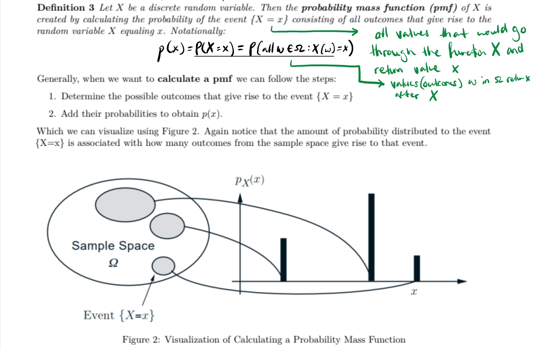
For Discrete cases we use Probability Mass Functions

Probability Mass Functions (PMF) — p(x)

Probability of an event {X = x} so all of the values that go into X and the output is x, these apply to continuous probability distributions

1) Determine the possible outcomes of some event
2) Add their probabilities to obtain p(x)

Bernoulli Random Variable: Explain and give shorthand

This is a random variable that only has two outcomes. Basically a yes or no situation.
X is either yes (1) if it’s in the category of interest or No (0) if not.

These 1 or 0 values are not fixed can be anything

Short hand: X ~ Bern(p) , X is defined by a Bernoulli distribution with parameter p

Parameters

inputs within the PMF that change the probability distribution

Binomial Experiment

This is just context, basically its a bunch of Bernoulli random variables together. n trails with either yes or no. AND each trail is independent and has the same probability of occurring.

Binomial Random Variable: Explain and give shorthand

X associated with a binomial experiment consisting on n trails and the function(X) is the number of success trails (x results in 1).
We want to figure out how many ways X can end up as success (matter the amount of trials and probability)

Shorthand : X ~ Bin(n,p)

Poisson Random Variable: explanation and shorthand

Type of data dealing with counts the pmf is given by (the image) and most likely values are around the parameter (λ)

X ~ Poisson (λ=1)

Probability Density Functions (pdf)

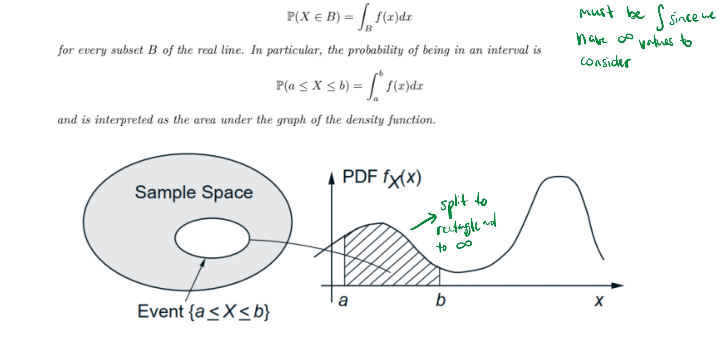
these are the continuous type of probability distribution functions of X.

X is continuous if there is nonnegative function (pdf) such that

for PDF since we are dealing with continuous the outer bounds do not matter since X cannot have a value for a single input (since we are talking about infinite values)

Support Set

the collection of possible values that X could be

Exponential Distribution

This is a common pdf with a scale factor of λ where λ is >0 if the pdf follows (image)

Normal Distribution - explain and give shorthand

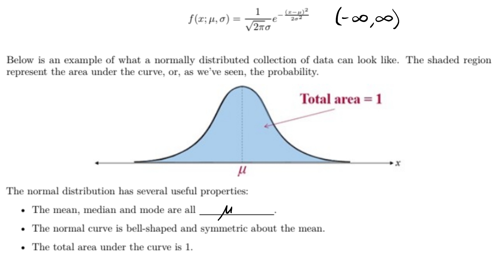
For a random variable X has a normal distribution with parameters μ (mean) and σ (standard deviation) if the density curve is (image) from (-inf,inf)

X ~ N(μ (center) , σ (scales))

Calculating Normal Distribution

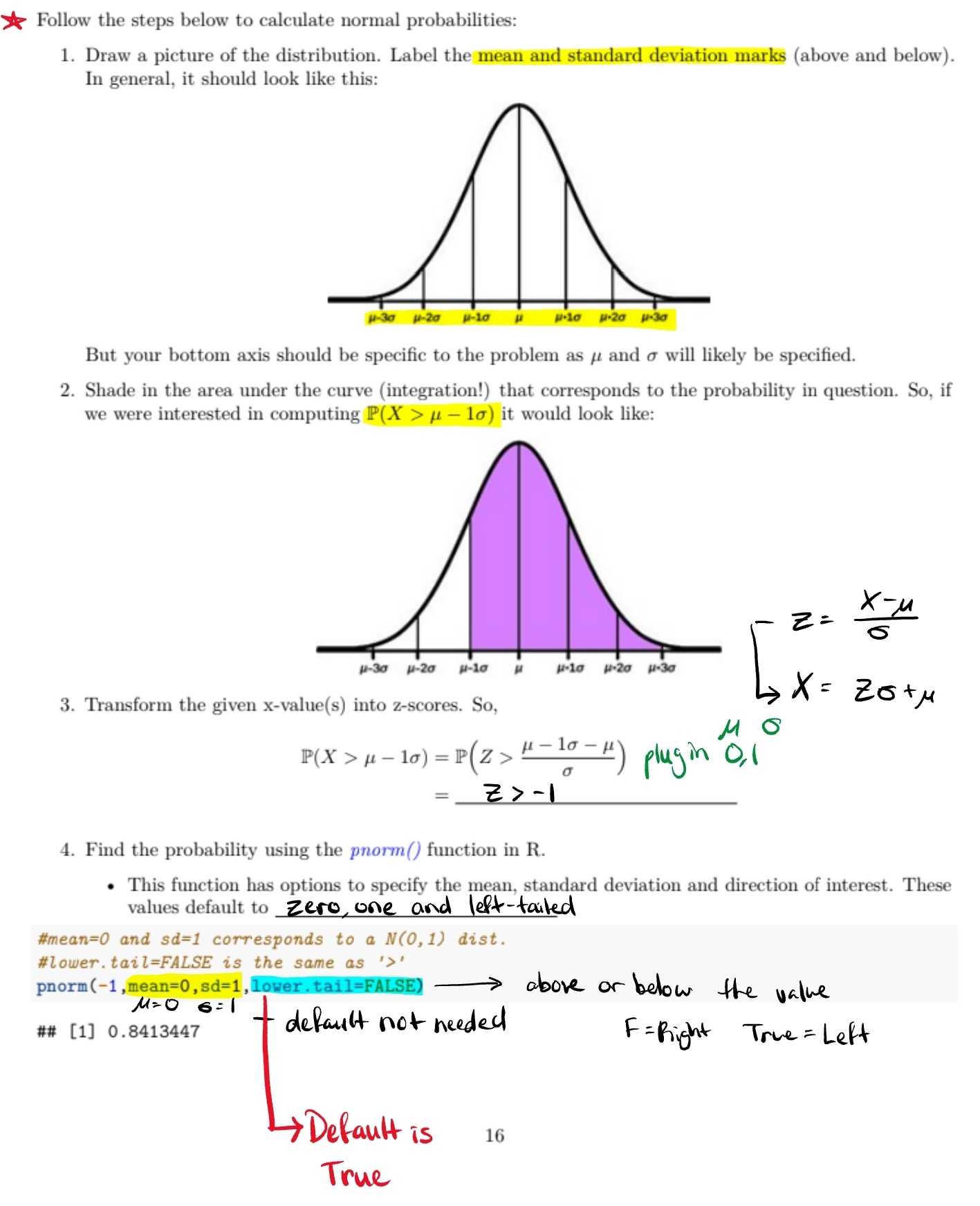
Instead of doing an integration (since it would take way too long and different for many values) we use a formalized way. Standard Normal Distribution, this means we keep the parameters 0,1 respectively.

We transform it into a Z-score

Z-Score

Z = X - μ/σ
(+) is above average

(-) is below average

We use this because the area under the curve (needed info) is the same for both

Solving Normal Distribution

Cumulative Distribution Functions (cdf)

These are used to come up with pmf and pdf from the CDF short of allow you to get values from the tables and subtract them (discrete) together or differentiate them (continuous).

No in between values so s step function with values from the tables of probabilities