Training Strategies and Augmentation Techniques for GNNs

Reasons and approaches of graph manipulation

1. Feature level:

• The input graph lacks features → feature augmentation

• Certain structures are hard to learn by a GNN (e.g. cycle count) → we add them as features

2. Structure level:

• The graph is too sparse = inefficient message passing
  → adding virtual nodes/edges

• The graph is too dense = message passing is too costly
  → random neighbor sampling

• The graph is too large = cannot fit the computational graph into a GPU
  → subgraph sampling for embedding computing

3. It is unlikely that the input graph happens to be the optimal computation graph for embeddings

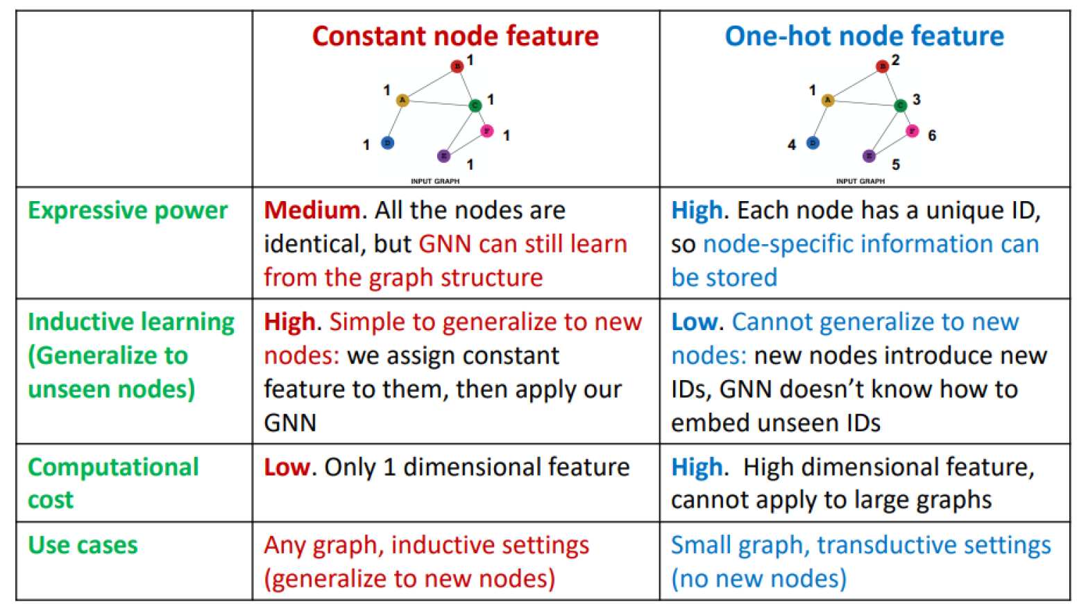
Feature augmentation approaches

• Assigning constant values to nodes

• Assigning unique IDs to nodes as one-hot vectors

• Adding certain features, e.g. centrality, clustering coefficient

Comparison of feature augmentation approaches

Common approach for adding virtual edges

Connecting 2-hop neighbors via virtual edges
→ using A+A² as computation graph

Use case: bipartite graphs (e.g. author-to-papers graph → 2-hop is author-to-author collaboration)

Method and benefit of adding virtual nodes

• The virtual node will connect to all the nodes in the graph → all nodes will have a maximum distance of 2

• Benefit: greatly improved message passing

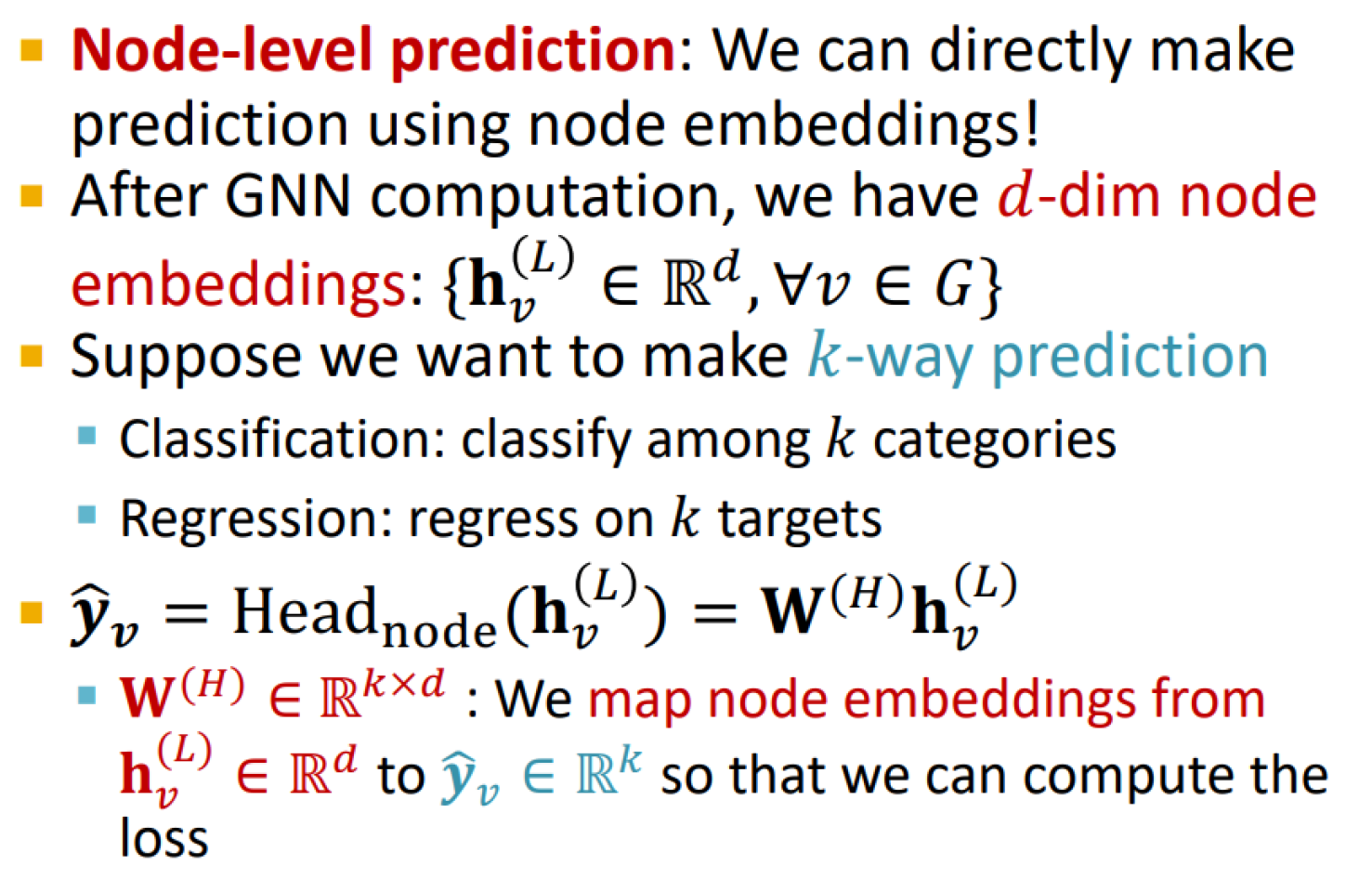
Node-level prediction head

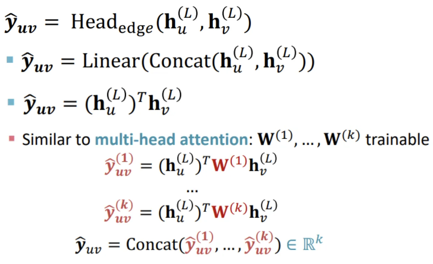
Edge-level prediction head

Make predictions using pairs of node embeddings.

Options:

• Concatenation + Linear layer: map 2d-dimensional embeddings to k-dimensional (k-way prediction)

• Dot product: simple dot product for one-way prediction, trainable W matrices for k-way prediction

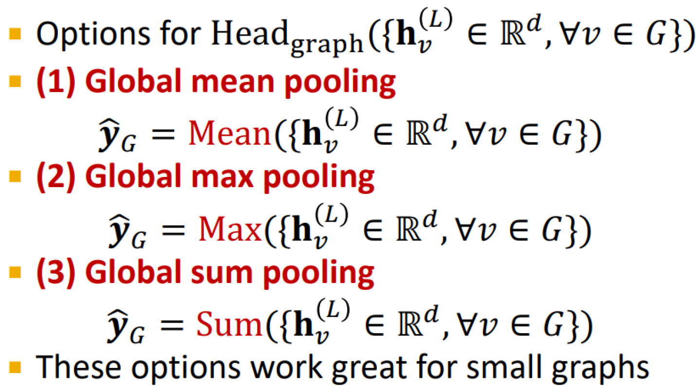
Graph-level prediction head

Make prediction using all the node embeddings in the graph

Unsupervised prediction task examples

• Node-level: node statistics, e.g. clustering coefficient

• Edge-level: link prediction

• Graph-level: deciding isomorphism of two graphs

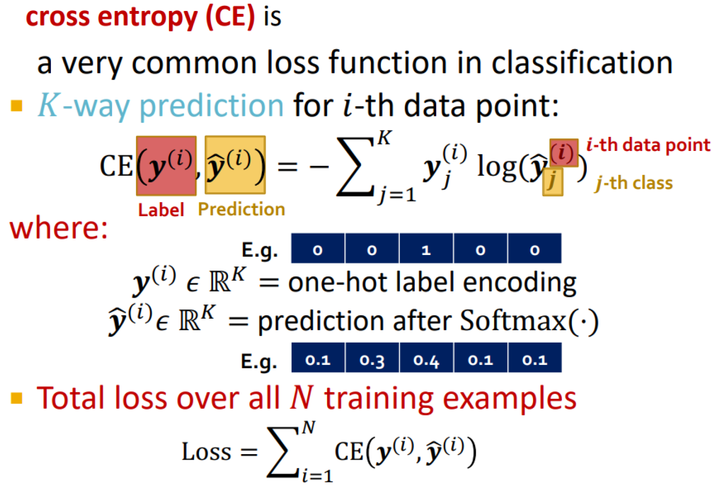
Classification loss

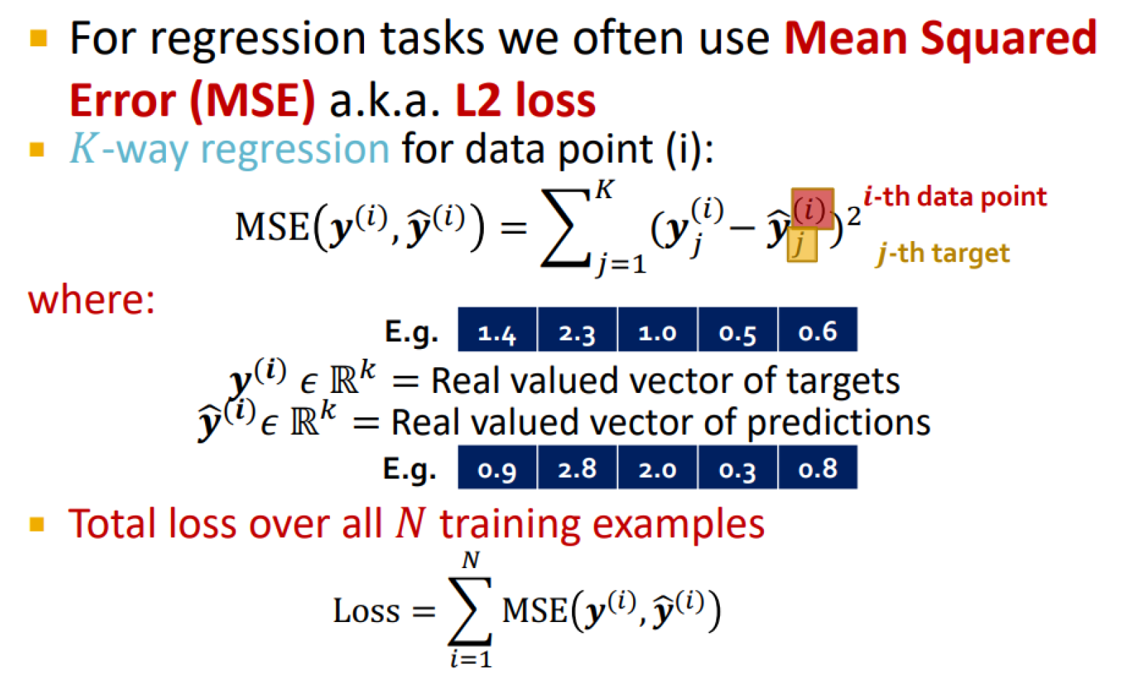
Regression loss

Fixed vs. random dataset split

• Fixed: we will split our dataset once

• Random: we randomly split, report average performance over different random seeds

Challenge of graph splitting

The nodes (data points) are not independent, they affect each other’s prediction

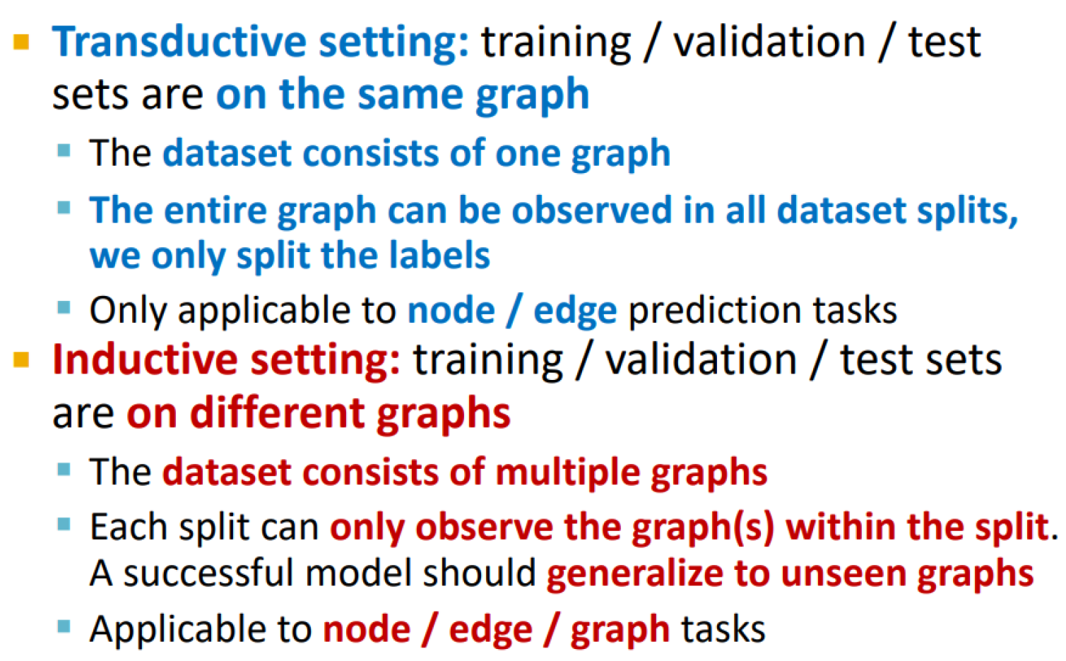
Transductive vs inductive splitting

Transductive link prediction

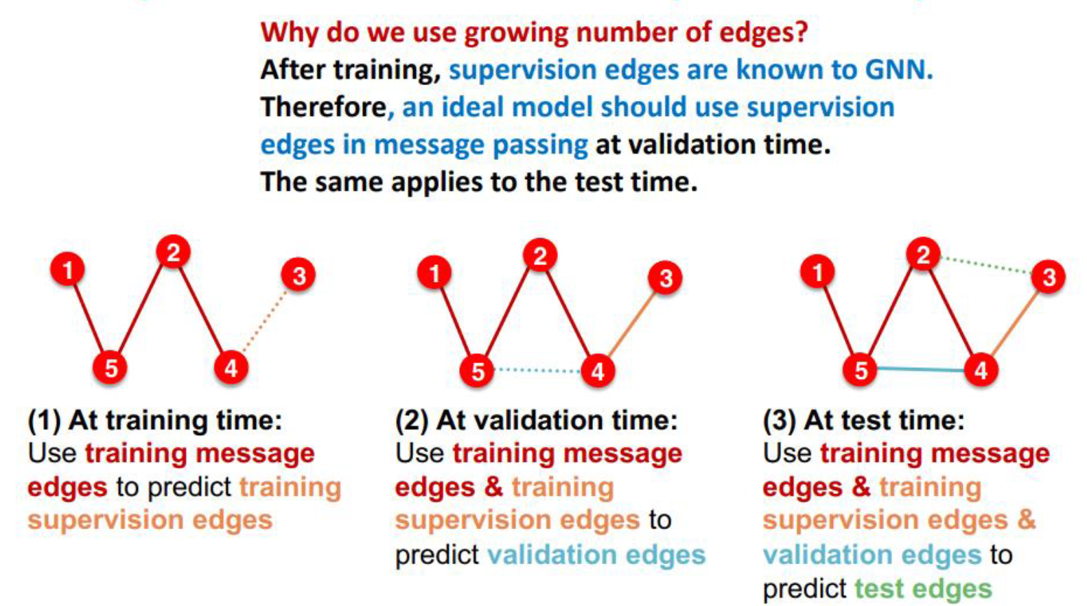
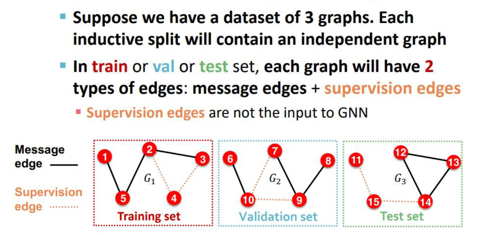
Inductive link splitting

Computational graph and its effect on node embeddings

Computational graphs are defined by the nodes’ neighborhood = rooted subtree structures around each node
→ if two nodes features and computational graphs are the same, the GNN won’t be able to distinguish them, they will get the same embeddings, since it doesn’t care about node IDs

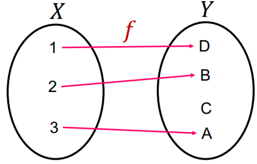
Injective function

It maps different elements into different outputs
→ retains all the information about the input

Most expressive GNN

Maps rooted subtrees to node embeddings injectively.
→ use an injective neighbor aggregation to fully retain the neighboring information and therefore distinguish different subtree structures

Expressive power, GCN and GraphSAGE case

Expressive power of GNNs can be characterized by that of neighbor aggregation function.

Neighbor aggregation is equivalent to a multi-set function

GCN:

• element-wise mean pool

• failure case: multi-sets with same color proportion

GraphSAGE:

• element-wise max pool

• failure case: multi-sets with same set of distinct colors

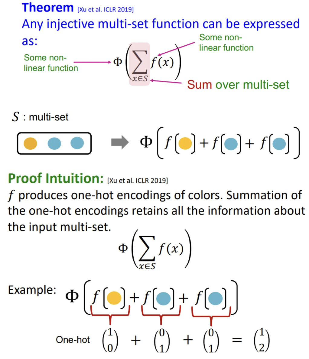
Injective multi-set function

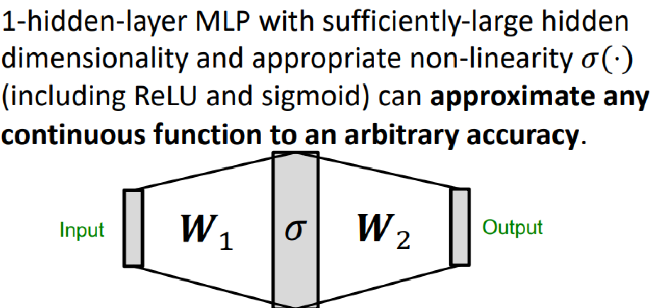
Universal approximation theorem

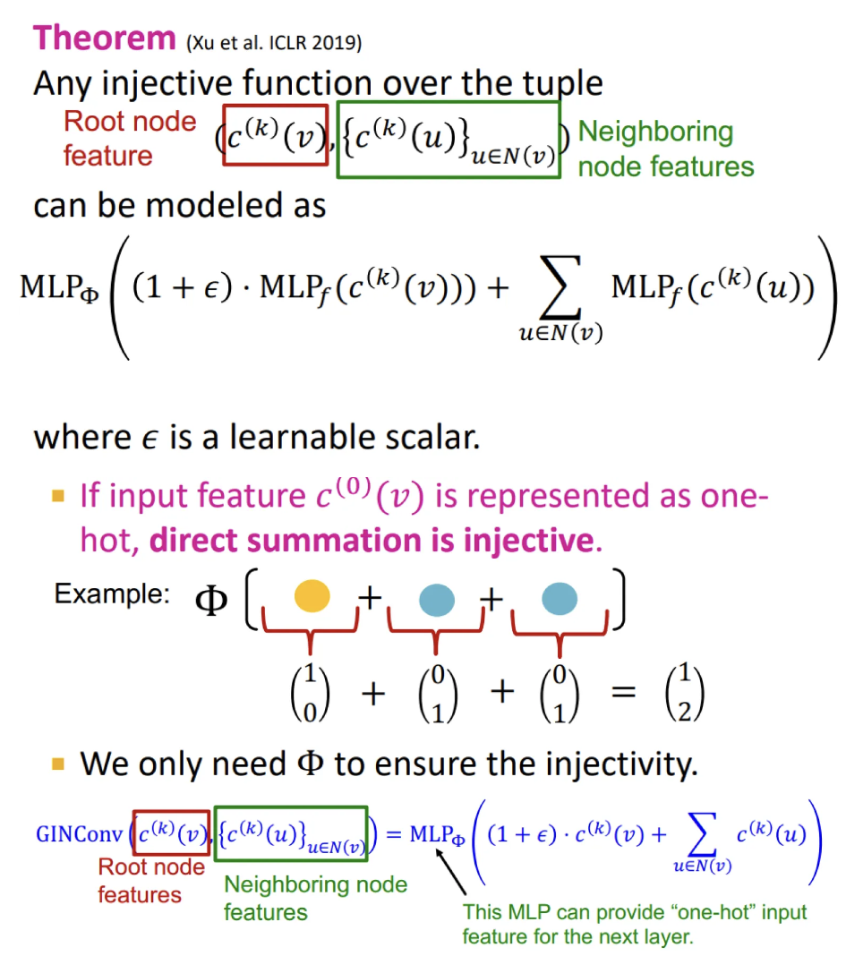
Graph isomorphism network (GIN)

A differentiable neural network version of the WL graph kernel:

• GIN uses a neural network to model the injective hash function

• GIN’s update targets are the node embeddings (low-dim vectors), not the one-hot node colors

=> their expressive power is the same, they can distinguish most of the real-world graphs

Advantages:

• Due to the low-dimensional node embeddings, they are able to capture fine-grained node similarity

• Parameters of the update function can be learnt for the downstream tasks

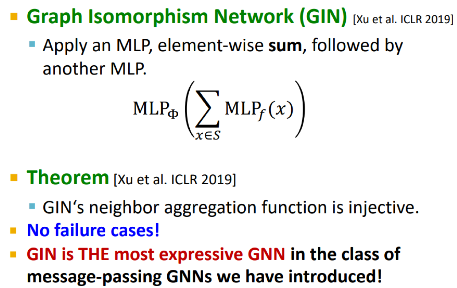
Injective function of GIN

Uses element-wise sum pooling instead of mean/max