Introduction to design part C

objective

the quantity to be maximized or minimized in an optimization problem

state the objective as a function of a finite set of variables

decision variables

first step in formulating the optimization problem

the objective function

quantification of uncertainty

an additional complication in formulating the objective function

variations introduced by unsteady plant operation, or imprecision in the design data and the constraint equations.

There may also be uncertainty in the decision variables, either from variation in the plant inputs,

Constraints on the optimization

the set of equations that bound the decision variables and relate them to each other

Equality constraints

arise from conservation equations and constitutive relations

any equation into the optimization model containing an ‘=’

Inequality constraints

arise from external constraints (safety, legal, market and econ, technical limits set by codes and standards, feed and prods specs, availability etc.)

limit the parameter space

effect of constraints is to

unbounded problems

the set of constraints does not bound the problem, approaches infinity (±), no maximum can be found

over-constrain the problem

does not contain any solution to the equality constraint

problem is infeasible

𝑛– 𝑚𝑒 degrees of freedom

the problem has 𝑛 variables and 𝑚𝑒 equality constraints

𝑛 = 𝑚𝑒

no degrees of freedom and the set of 𝑚𝑒 equations can be solved for the 𝑛 variables

𝑚𝑒 > 𝑛

the problem is over-specified

and hence reduce the space in which the search for the optimum is carried out.

that inequality constraint becomes an equality and is said to be “active”.

When inequality constraints are introduced into the problem, they generally set bounds on the range over which parameters can be varied

If the behavior of a system is well understood, then the design engineer can decide that an inequality constraint is likely to be active

It is often possible to use engineering insight and understanding of chemistry and physics to simplify the optimization problem.

he number of degrees of freedom is reduced by one and the problem is made simpler.

By converting the inequality constraint into an equality constraint,

Inexperienced engineers are often unaware of many constraints and consequently find “optimal” designs that are dismissed as unfeasible by more experienced designers.

The correct formulation of constraints is the most important step in setting up an optimization problem.

determined by a trade-off between two or more effects

If the optimal value of the objective is not at a constraint limit then it will usually be

If the minimum temperature approach is increased then the capital cost is reduced but less energy is recovered.

A high degree of heat recovery requires close temperature approaches in the heat exchangers, high capital cost as the exchangers require more surface area.

The optimum value of the approach temperature, ∆𝑇𝑜𝑝𝑡𝑖𝑚𝑢𝑚, is then given by the minimum point in the total cost curve.

If the capital cost is annualized then the two costs can be added to give a total cost.

• More separations equipment and operating cost vs. lower product purity

• More recycle costs vs. increased feed use and waste formation

• More heat recovery vs. cheaper heat exchange network

• Higher reactivity at high pressure vs. more expensive reactors and higher compression costs

• Fast reactions at high temperature vs. product degradation

• Marketable byproducts vs. more plant expense

• Cheaper steam and electricity vs. more off-site capital cost

The task can be reduced by dividing the process into more manageable units, identifying the key variables and concentrating work where the effort involved will give the greatest benefit.

The task of formally optimizing the design of a complex processing plant involving several hundred variables, with complex interactions, is formidable

Care must always be taken to ensure that sub-components are not optimized at the expense of other parts of the plan

he optimization of one unit may be at the expense of another.

• If the second derivative of the objective function is greater than zero at a stationary point then the stationary point is a local minimum.

• If the second derivative is less than zero then the stationary point is a local maximum.

• If the second derivative is equal to zero then it is a saddle point.

• If the objective is a function of a single variable, 𝑥, the objective function 𝑓(𝑥) can be differentiated with respect to 𝑥 to give 𝑓’(𝑥).

• Any stationary points in 𝑓(𝑥) can then be found as the solutions off 𝑓’(𝑥).

• If 𝑥 is bounded by constraints, then we must also check the values of the objective function at the upper and lower limiting constraints.

• Similarly, if 𝑓(𝑥) is discontinuous, then the value of 𝑓(𝑥) on either side of the discontinuity should also be checked.

the objective function very often can not be written as a simple equation that is easily differentiated.

true when the objective function requires solving large computer models, possibly using several different programs and requiring several minutes, hours or days to converge a single solution.

he optimum is found using a search method.

Unrestricted Search

If the decision variable is not bounded by constraints then the first step is to determine a range in which the optimum lies.

an unrestricted search an initial guess of 𝑥 is made and a step size, ℎ, is assumed.

followed by calculations of 𝑧1 = 𝑓(𝑥), 𝑧2 = 𝑓(𝑥 + ℎ), and 𝑧3 = 𝑓(𝑥 − ℎ).

the values of 𝑧1, 𝑧2, and 𝑧3 the direction of search is determined that leads to improvement in the value of the objective, depending on whether 𝑧 is be to minimized or maximized.

𝑥 is then continuously increased (or decreased) by successive steps of ℎ until the optimum is passed.

a relatively simple method of bounding the optimum for problems that are not constrained

Once a restricted range that contains the optimum has been established, restricted range search methods can be used.

These can be broadly classified as direct methods that find the optimum by eliminating regions in which it does not lie, and indirect methods that find the optimum by making an approximate estimate of 𝑓’(𝑥).

Regular Search

By eliminating two of the four quarters of the range at each step, this procedure reduces the range by half each cycle.

• To reduce the range to a fraction 𝜀 of the initial range therefore takes 𝑛 cycles, where 𝜀 = 0.5 𝑛 . • Since each cycle requires calculating 𝑓(𝑥) for two additional points, the total number of calculations is 2𝑛 = 2 log 𝜀 / log 0.5.

• The procedure is terminated when the range has been reduced sufficiently to give the desired precision in the optimum.

• For design problems it is usually not necessary to specify the optimal value of the decision variables to high precision, so 𝜀 is usually not a very small number.

Golden Section Search

Called the golden mean search,

implement as the regular search, but is more computationally efficient if 𝜀 < 0.29.

Start by evaluating 𝑓(𝑥𝐿) and 𝑓(𝑥𝑈) corresponding to the upper and lower bounds of the range, labelled 𝐴 and 𝐵 (Fig. 1.12).

• Add two new points, labelled 𝐶 and 𝐷, each located a distance 𝜔𝐴𝐵 from the bounds 𝐴 and 𝐵, i.e., located at 𝑥𝐿 + 𝜔(𝑥𝑈 − 𝑥𝐿) and 𝑥𝑈 − 𝜔(𝑥𝑈 − 𝑥𝐿).

• For a minimization problem, the point that gives the highest value of 𝑓(𝑥) is eliminated (point 𝐵 in Fig. 1.12).

• A single new point, 𝐸, is added, such that the new set of points 𝐴𝐸𝐶𝐷 is symmetric with the old set of points 𝐴𝐶𝐷𝐵.

Quasi-Newton Search

Newton’s method is a super-linear indirect search method that seeks the optimum by solving 𝑓’(𝑥) and 𝑓’’(𝑥) and searching for where 𝑓’(𝑥) = 0.

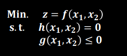
two-variable optimization problem can be stated as

For simplicity, all problems will be stated as minimization problems from here on.

• A maximization problem can be rewritten as 𝐌𝐢𝐧. 𝒛 = −𝒇 𝒙𝟏, 𝒙𝟐 .

Convexity

If the constraints are not linear, then there is a possibility that the feasible region may not be convex.

A convex feasible region is one in which any point on a straight line between any two points inside the feasible region also lies within the feasible region.

Problems with a convex feasible region are more easily solved to a global optimum.

Problems with non-convex feasible regions are prone to convergence to local minima.

univariate search

If 𝑥1 and 𝑥2 are varied one at a time then the method is known as a ______- and is the same as carrying out successive line searches.

the steepest descent method

the gradient method)

probabilistic methods

such as simulated annealing or genetic algorithms that introduce some possibility of moving away from a local optimum

the problem of convergence to a local optimum, wherein different answers are obtained for different initial solutions. Can be overcome by using pattern searches with a larger grid or by using

A set of continuous linear constraints

defines a convex feasible region.

If the objective function is also linear and 𝑥𝑖 > 0 for all 𝑥𝑖 , then the problem can be written as a linear program (LP)

can be used to solve very large problems, with thousands of variables and constraints.

widely used in operations, particularly in optimization of oil refineries and petrochemical plants

vertex of the feasible region.

The optimum must lie on the boundary at an intersection between constraints

always solve to a global optimum

Many algorithms have been developed for solution of linear programs, of which the most widely used are based on the SIMPLEX algorithm developed by Dantzig (1963).

The SIMPLEX method introduces slack and surplus variables to transform the inequality constraints into equalities.

The resulting set of equalities is solved to obtain a feasible solution, in which some of the slack and surplus variables will be zero, corresponding to active constraints.

the contours of the objective function are exactly parallel to one of the constraints.

• The problem is said to be degenerate and has an infinite number of solutions along the line of that constraint.

• Linear programming can be used to solve very large problems, with thousands of variables and constraints.

• The method is widely used in operations, particularly in optimization of oil refineries and petrochemical plants.

• It is used a lot less in design, as design problems almost inevitably contain many non-linear equations.

Successive linear programming (SLP)

Successive quadratic programming (SQP)

Reduced gradient method

Three main methods are used for solving a NLP: