CS 234 Module 9: Improvements

Average case

A calculation of running time in which the representative value for each instance size k is determined by taking the sum over all instances of that size of the product of the probability of the instance and its running time

What is the formula for average-case running time?

∑_I∈S Pr[I] ∙ Cost(I)

• I ∈ S: Possible data items

• Pr[I]: Probability of a particular data item being sought

• Cost(I): Cost for searching for a particular data item

Uniform Distribution

• All probabilities are equal

• Probability for each item = 1/n

• For successful search, n is the number of data items stored

• For unsuccessful search, n is the number of data items that might be sought

Cost of Finding a Data Item

At most n data items need to be examined to find any data item, that is: Cost[I] ≤ n for each data item I

Upper Bound of Linear Search

Total = O(n)

∑_I∈S Pr[I] ∙ Cost(I) ≤ ∑_I∈S 1/n ∙ n ∈ O(n)

Lower Bound of Linear Search

Total cost: Ω(n),

using the fact that there are at least ⌊n/2⌋ data items in the second half of the array, so for each I∈T, Cost(I) ≥ ⌊n/2⌋

∑_I∈S Pr[I] ∙ Cost(I) ≥ ∑_I∈T Pr[I] ∙ Cost(I) = ∑_I∈T 1/n ∙ Cost(I) ≥ ∑_I∈T 1/n ∙ ⌊n/2⌋ ≥ ⌊n/2⌋ ∙ 1/n ∙ ⌊n/2⌋ ∈ Ω(n)

Cost of Searching A Node in Tree

Cost[I] ≤ log n

Cost of searching is linear in tree depth; since the height of the tree is logarithmic, no data item is in a node of depth greater than logarithmic.

Upper Bound of Binary Search

Total = O(log n)

∑_I∈S Pr[I] ∙ Cost(I) ≤ ∑_I∈S 1/n ∙ log n ∈ O(log n)

Lower Bound of Binary Search

Total cost: Ω(log n),

Using the line we drew, each node below the line is at least halfway down the tree; each data item in T requires at least ⌊(log n)/2⌋ time, so Cost(I) ≥ ⌊(log n)/2⌋

Since at least half the data is in T, |T| ≥ ⌊(log n)/2⌋.

Multiplying roughly half by roughly half = roughly a quarter, which is in Ω(log n)

∑_I∈S Pr[I] ∙ Cost(I) ≥ ∑_I∈T Pr[I] ∙ Cost(I) = ∑_I∈T 1/n ∙ Cost(I) ≥

∑_I∈T 1/n ∙ ⌊(log n)/2⌋ ≥ ⌊n/2⌋ ∙ 1/n ∙ ⌊(log n)/2⌋ ∈ Ω(log n)

What is the Worst-Case Cost of Linear Search?

θ(n)

What is the Worst-Case Cost of Binary Search?

θ(log n)

Improved Binary Search

At each phase of binary search in array A:

• Consider positions Low through High

• Mid = Low + 0.5(High - Low)

• At each phase, Data is compared to A[Mid]

• If Data is bigger:

  • Update Low = Mid + 1

• Otherwise:

  • Update High = Mid - 1

Interpolation Search

At each phase of binary search in array A:

• Consider positions Low through High

• Mid = Low + (Data-A[Low])/(A[High]-A[Low]) ∙ (High - Low)

  • Low + weight x size of interval

• At each phase, Data is compared to A[Mid]

• If Data is bigger:

  • Update Low = Mid + 1

• Otherwise:

  • Update High = Mid - 1

What is the average-case runtime of Interpolation Search?

O(loglog n), when the data is evenly spaced

What is the worst-case runtime of Interpolation Search?

θ(n)
In the worst case, we could choose a value of Mid that splits the interval into a piece of size one and a piece of size one less than the original interval, and end up having to search in the bigger piece.
This can happen in every phase

Heuristic

A method that may not guarantee bounds on running time or correctness

Uniform Distribution

A probability distribution in which all probabilities are equal

What is the calculation for the average-case cost of a successful search, given that:

• we have a uniform distribution, and

• the cost of finding an item in position 𝔦 is the number of items that need to be read (𝔦 + 1)

(n+1)/2

What is the average cost of a search if the data items are stored in the order ape, cat, dog, and pig?

Cost(Ape)*Pr(Ape) + Cost(Cat)*Pr(Cat) + Cost(Dog)*Pr(Dog) + Cost(Pig)*Pr(Pig)

= 1 × 1/8 + 2 × 1/4 + 3 × 1/8 + 4 × 1/2
= 1/8 + 1/2 + 3/8 + 2
= 3

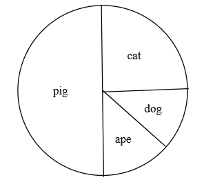
How does cost change in linear search on an array?

The cost of linear search in slot 0 is 1, and increases by 1 as slot number increases by 1

What strategy should be used to obtain the smallest worst-case cost for linear search?

Put the items in nonincreasing order of probability. Doing so results in higher probabilities being multiplied by smaller costs.

Self-organizing Heuristic

Use information about past accesses to rearrange data items

Move to Front Herustic

Based on the assumption that if a data item is accessed, it is likely to be accessed again. Rearrangements are hoped to help bring down the cost of future searches of searched items.

• Linear search for the item

• After a successful search, move the item that was sought to the front of the list

• Consequently, each data item before that sought item is moved one position closer to the back of the list

• Most-searched element moves to the front quickly, slipping back each time another item is accessed

• Least-searched element moves one closer to the back each time an element after it is accessed

Transpose Heuristic

A less disruptive heuristic than Move to Front

• Linear search for the item

• After a successful search, exchange the found data item with the preceding data item, if any

• The most-searched element moves slowly to the front, and the least-used element moves slowly to the back

When does Transpose outperform Move to Front?

Transpose does better than Move to Front unless:

• there are only two items

• all items are equally probable to be sought

Digital Data

A way of ADTs treating data items, using functions that extract information from data items

Bit Vector

A data structure consisting of a single bit for each data item, taken from a fixed range of integers. Data items are stored as 1s.

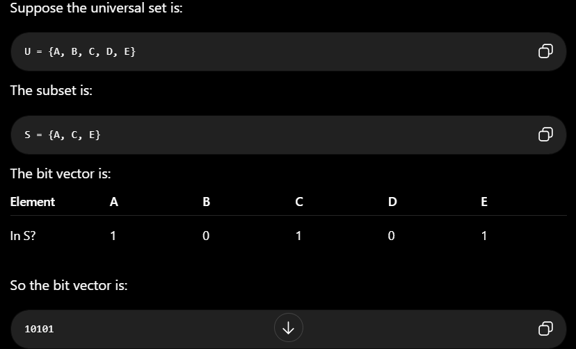
What is the runtime for search in a bit vector?

It takes constant time due to random access.

Hashing

A general way of mapping keys to integers in the range, aka distributing keys into buckets.

What does all methods of hashing have in common?

Each method specifies a hash function ⨍, and a method for collision resolution.

Hash Function ⨍

Maps keys (or data items) to buckets.

Each key is mapped to a value in the range from 0 to N-1, where N is the number of buckets

Collision

Occurs when 2 different keys are mapped by the hash function ⨍ to the same bucket

Types of Conflict Resolution

Separate chaining and open addressing.

Separate Chaining

Make each bucket big enough to store all data items that are mapped to it; by storing all data items k with ⨍(k) = i in bucket i

Algorithm for ADT Dictionary CREATE for Hashing

Initializes any data structure (typically an array) used in hashing.

Algorithm for ADT Dictionary IS_EMPTY for Hashing

Require checking all array entries, unless an implementation includes a variable used to keep track of the number of data items stored.

Algorithm for ADT Dictionary LOOK_UP for Hashing

Varies substantially depending on the type of hashing.

Algorithm for ADT Dictionary ADD for Hashing

Consists of the same algorithm as LOOK_UP, followed by either

• replacing the element (if a data item with the key being sought has been found), or

• inserting the new data item in the appropriate location

Algorithm for ADT Dictionary DELETE for Hashing

Consists of the same algorithm as LOOK_UP, but unlike in the case of adding a data item, additional steps might be required to ensure that future LOOK_UP operations will work properly.

How to measure the cost of search for a data item?

As the number of probes needed to find data item. Where each probe is the examination of a data item or location

Load Factor

The ratio of the number of data items to the number of buckets

The average number of probes needed for a search is compared to this for a particular type of hashing

Bit

0 or 1

What are the goals for hash functions?

1. Quick to compute, since we need to compute the function every time we search for a data item

2. Spread keys evenly among buckets to reduce collisions

Modular Arithmetic

a system of arithmetic where numbers wrap around after reaching a certain value, called the modulus.

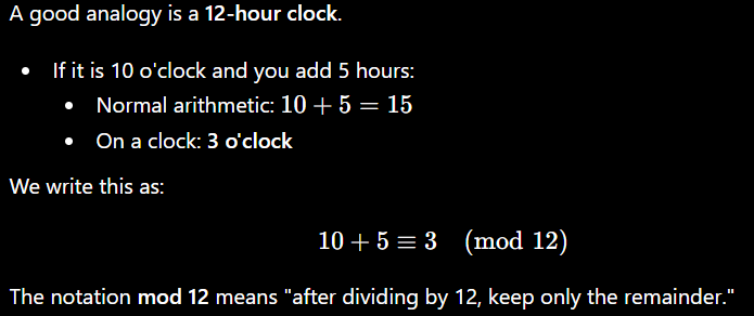
Hash Function Example 1: f(k) = ⌈log N⌉ Leading/Trailing bits in k as binary number

• A quick-to-compute function by extracting bits using division

• Doesn’t spread keys evenly among buckets.

  • If keys are strings, this hash function may categorize strings by the first/last letter. Not all letters appear with equal frequency in a language, resulting in an uneven distribution of keys in buckets

Hash Function Example 2: Modular Arithmetic

• f(k) = k mod N

• A quick-to-compute function

• Not necessarily spread keys evenly among buckets

  • If N (number of buckets) is a power of 2, this is the same as Example 1 with strings as keys

Hash Function Example 3: f(k) = (ak + b) mod N for each value of k

Uses randomness to try to break up any patterns in the data.
a and b are selected at random, and then the same values of a and b are reused

Goals of Hashing

1. The hash function distributes keys among buckets as evenly as possible.

2. The hash function does not take a lot of time to compute.

3. Collision resolution minimizes the average number of probes required.

4. Collision resolution does not take a lot of time to compute.

Probes

The examination of a data item or location in hashing

Dictionary Hashing using Separate Chaining Linked List Implementation

Data structures:

• Array in which each slot stores the null pointer or a pointer to a linked list of nodes, each storing a data item and a pointer Next to the next linked node in the list, if any, and otherwise the null pointer

Definition:

• The linked list for slot i forms bucket i.

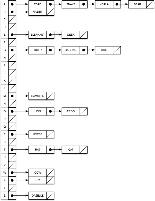
LOOK_UP(D, Key) under Dictionary Hashing using Separate Chaining Linked List Implementation

Worst-case cost: θ(n)

1. Use the hash function on Key to determine which slot Key belongs in

2. Linear search of linked nodes until Key or the last linked node is found

   1. Return the element stored with Key

   2. Return false otherwise

ADD(D, Key, Element) under Dictionary Hashing using Separate Chaining Linked List Implementation, where Key is guaranteed to use a key that isn’t used for any data item.

Worst-case cost: θ(1)

1. Use the hash function on Key to determine which slot Key belongs in

2. Allocate a new linked node Node storing Key and Element

3. Add Node to the beginning of the linked list

DELETE(D, Key) under Dictionary Hashing using Separate Chaining Linked List Implementation

Worst-case cost: θ(n)

1. Use the hash function on Key to determine which slot Key belongs in

2. Linear search of linked nodes until Key is found

3. Remove the node storing Key

Worst-case cost of CREATE() under Dictionary Hashing using Separate Chaining Linked List Implementation

The array can be allocated in constant time. Each slot can be initialized in constant time, for a total in θ(N) time.

N = number of buckets

Worst-case cost of CREATE() under Dictionary Hashing using Separate Chaining Linked List Implementation

Each of the N slots can be read in constant time, for a total in θ(N) time.

N = number of buckets

ADD(D, Key, Element) under Dictionary Hashing using Separate Chaining Linked List Implementation, where Key might be used by data item that is currently stored in the ADT.

Worst-case cost: θ(n)

1. Use the hash function on Key to determine which slot Key belongs in

2. Linear search of linked nodes until Key or the last linked node is found

   1. If Key is found, update the pair to store Element

   2. If Key is not found,

      1. Allocate a new linked node Node storing Key and Element

      2. Add Node to the beginning of the linked list

What counts as a probe for separate chaining?

Each read of a slot in the array and each read of a linked node counts as a probe.

Open Addressing

• Each bucket is associated with a slot in an array.

• Store at most one item in each bucket.

• A data item k might not be stored in the bucket f(k).

• ADD, LOOK_UP, and DELETE search through slots in a particular order for a particular data item.

Probe Sequence for a Data Item

The order of buckets the algorithm examines until it finds the key or an empty slot.

Algorithm of LOOK_UP for a Probe Sequence

1. Checking buckets in the order of the probe sequence

2. In a successful search: search stops when a data item is found

3. In an unsuccessful search: search stops as soon as an empty bucket is found

Algorithm of ADD for a Probe Sequence

1. Checking buckets in the order of the probe sequence

2. If a data item with the sought key is found:

   1. Stops search

   2. Update element

3. If the key is not found:

   1. Allocate a new data item

   2. Insert the new item in the first empty bucket we found

Why the Algorithm of DELETE for a Probe Sequence is so complex and outside of the scope of this course.

When a data item α is stored later in the probe sequence after a data item is deleted. If the deleted item leaves an empty bucket, a future search for α will stop at that empty bucket rather than continue searching for α.

What are the different methods of hashing that uses open addressing by specifying different rules about how to define the probe sequences for data items?

• Linear probing

• Quadratic probing

• Double hashing

Linear Probing

When adding a new data item with key κ,

1. if slot ⨍(κ) is full

2. we look at the next slot

3. and the slot after that

4. and so on…
   (including wrapping back to the beginning of the array ~ mod N)

5. stopping when we found an empty slot

6. Placing the new data item in the slot

Probe Sequence for κ: ⨍(κ), (⨍(κ)+1) mod N, (⨍(κ)+2) mod N,(⨍(κ)+3) mod N, so on

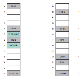
Clustering

A phenomenon in which once a collision occurs, more collisions tend to pile up in the same place, like a snowball growing bigger and bigger.

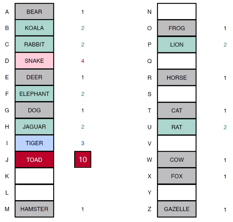
Quadratic Probing

Using squares for ‘step’ sizes, the probe sequence for κ:
⨍(κ), (⨍(κ)+1²) mod N, (⨍(κ)+2²) mod N, (⨍(κ)+3²) mod N, so on

What is the tradeoff in choosing probe sequences?

• Making probe sequences differ for different keys might reduce the chances of clustering.

• Making probe sequences differ for different keys might add to the cost of determining sequences.

Double Hashing

Forms different probe sequences even for keys where ⨍ maps to the same bucket by using a second hash function 𝔤(κ), the probe sequence for κ:

⨍(κ), (⨍(κ)+𝔤(k)) mod N, (⨍(κ)+2𝔤(k)) mod N, (⨍(κ)+3𝔤(k)) mod N, so on

How to choose 𝔤(k) to prevent some buckets from never appearing in any probe sequence?

• Make the number of slots (N) a prime number

• If and are not relatively prime, then and N have a common divisor d≠1.

• If there is such a d, then
  (⨍(κ)+(N/d) × 𝔤(k)) mod N = (⨍(κ)+ N × 𝔤(k)/d) mod N = ⨍(κ)

• Our probe sequence starts to repeat after only N/d steps, so we don't reach all the buckets

What are the differences of Open Addressing to Separate Chaining

Open Addressing

• uses array directly

• no extra space for pointer

• losing the flexibility of linked data

• fixed number of slots and a limit on the number of data items we can store

How to fix the problem where deleting an item leaves a gap, where linear search might stop before all data items in the probe sequence are checked?

We could solve that problem by viewing each slot as storing compound data, where one of the fields is a single bit that indicates whether or not the slot had ever contained a data item. That would us allow us to refill the slot, and in the interim to ensure that searches would not stop prematurely.

Bit Vector Algorithm

• Initializes each entry in the bit vector to 0.

• For each data item i, enters a 1 in index i.

• Creates a sequence by linear search through the slots, adding the index of each slot that contains a 1.

What is the worst-case running time of bit vector algorithm?

θ(n + r)

n = number of data items

r = range

ADT Bucket

Supports adding data items and returning contents in a bucket.

ADD_TO_BUCKET(B, Data)

Adds Data to bucket B

RETURN_CONTENTS(B)

• Returns all data items in bucket B

• Empties all contents in B

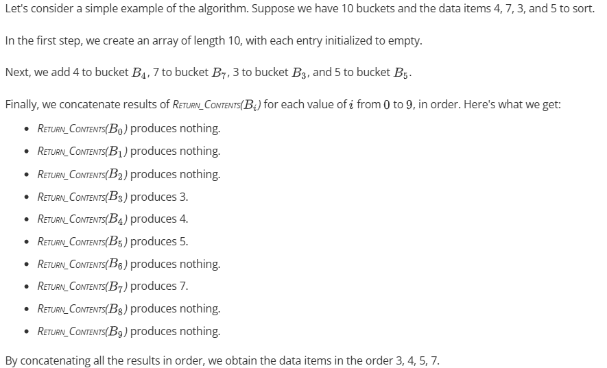
Bucket Sort

Using an array of r buckets named B₀ through B_r-1:

• Initializes each entry in an array of length r to empty in θ(r).

• For each data item (i, Value), executes ADD_TO_BUCKET(B_i, Value) in θ(n).

• For each bucket in order, concatenates the results of RETURN_CONTENTS(B_i) in θ(n + r).

What are the problems that arise with large values of r?

1. If r > n log n, there is no improvement over Heapsort’s runtime of θ(n log n)

2. If r is really large as f(n), the number of bits per value (log r) is very large.

   • Finding a slot will not be considered a θ(1) operation

Stable Sort

A sorting algorithm that does not change the order of equal-valued items.

A Pass

One complete traversal of the data during which the algorithm performs its intended comparisons and, if necessary, swaps or moves elements.
e.g.

• Sort by day of the month

• Sort by month

• Sort by year