E300 Key Definitions and Formulae

FGLS process (multiplicative heteroskedasticity)

See slides + notes

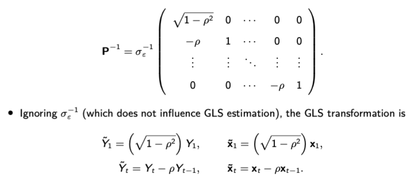
Cochrane Orcutt + Prais Winsten FGLS (serial error correlation)

1. Run OLS on Y = Xbeta + epsilon to obtain residuals

2. Estimate an AR coefficient by regressing residuals at t on residuals at t-1

3. Perform the pictured GLS transformation with your estimated p

4. Run OLS on the transformed data

This is Prais-Winsten estimation, if we ignore the first observation which needs a different transformation, we run the Cochrane-Orcutt procedure.

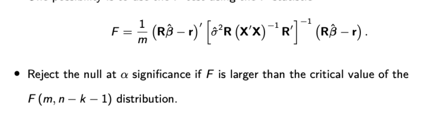
Formula for F statistic

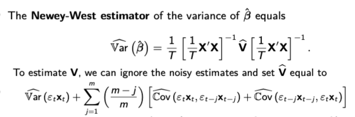
Newey-West variance estimator

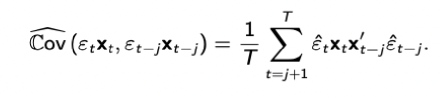
Noisy for large j, but good for small j

GLS

With heteroskedasticity, the conditional error variance will be some function of X. To remove it, denote P as the ‘square root’ of that funciton, then transform each variable by dividing it by P. Running the transformed regression will give a conditional error variance of 1.

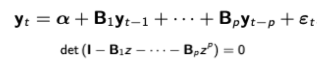
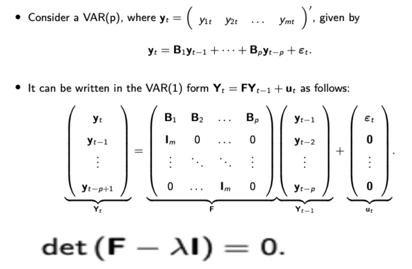
Stationarity of VAR(p)

From the pictured VAR(p) model, stationarity is ensured when all roots of the lag polynomial expression (below) are greater than one in absolute value.

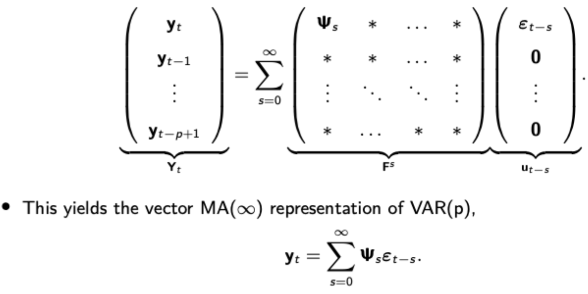
Vector MA(inf) and impulse response functions

Like in AR(1), VAR(1) can be represented in vector MA(inf) form, pictured. The top-left mxm block of F^s is the impulse response function.

The i-th row and j-th column of this mxm block can be interpreted as the effect of a one unit increase in the j-th component of ‘s-th’ lag of the errors on the i-th component of y at t. The response is dynamic, hence different effects on y over time.

The impulse response function can also describe the plot over time of the response of the i-th component of y at t+s to a one time impulse in the j-th component of the error term at t.

Strict and weak stationarity

Strict stationarity: (yt and yt+s) have the same joint distribution for all t and s

Weak stationarity: Mean and variance are time invariant, and the covariance function depends only on the lag (not on the time)

Calculating variance, autocovariance and autocorrelation for an AR(1) process (finite and infinite time)

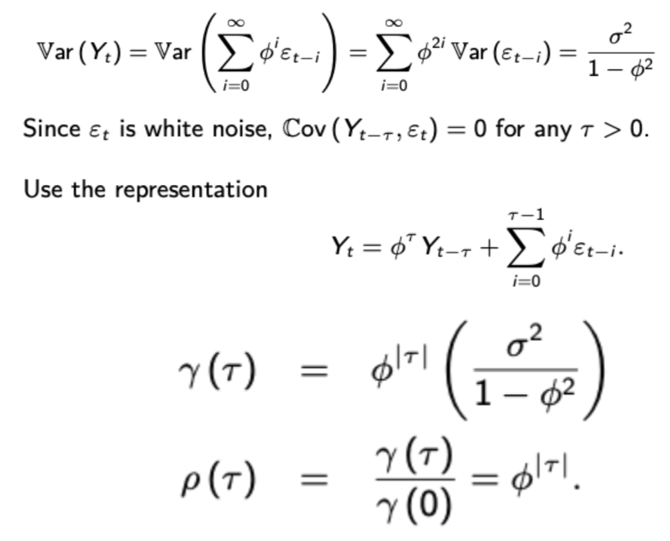
Represent your stable AR(1) as MA(inf) (Wold representation), then use this to find variance, autocovariance and autocorrelation. In the finite past, this can still be stationary so long as we assume that the initial condition (Y0) is distributed with 0 mean and the same variance as pictured for the infinite past.

Calculating variance, autocovariance and autocorrelation for an MA(q) process

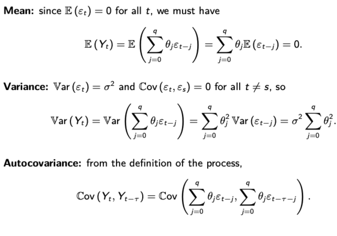
Autocovariance just becomes the pairs of coefficients that have overlap (i.e. if the lag is 1 and there it is MA(3), there will be overlap in the t-1, t-2, and t-3 terms.

Invertibility and the difference between it and stationarity

Stationarity means that the MA interpretation of AR converges, so you can write your AR process Y as MA (in terms of the movements of its errors). This is true if the roots of your lag polynomial are all greater than one in absolute value.

Invertibility means that your MA model can be inverted so that your errors are written in terms of the current and past values of Y. Again, this ensures that a unique model can be fit to the data. It also requires parameters to be inside the unit circle, but for the inverse roots of the MA polynomial.

Summing up AR / MA / ARMA processes

AR(1) + AR(1) = ARMA(2,1)

AR(1) + White noise process = ARMA(1,1)

MA(1) + MA(1) = MA(1)

Where all processes on the left side are uncorrelated at all lags and leads. This is useful because it allows aggregation of individual AR(1) processes

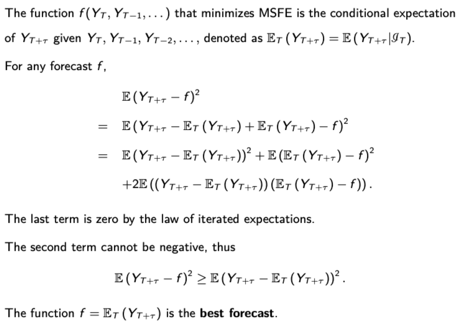
Optimal forecasting

Minimises mean squared forecast error, proof shown

OLS consistency in FDL models (but not autoregression)

• No multicollinearity

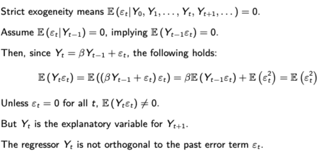
• Strict exogeneity conditional expectation of the error term given all past, present and future values of X is 0

Why does strict exogeneity fail for AR processes

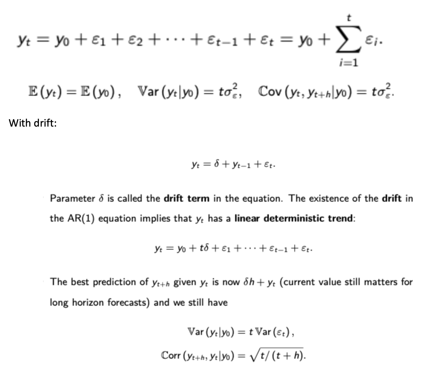
Calculating autocorrelation functions, variance, and autocovariance for random walks, with and without drift

Unit roots, difference and trend stationarity

Unit root: Lag polynomial has one root on with an absolute value of 1 (on the unit circle)

Difference stationary: Becomes stationary after first differencing (i.e. the difference between a variable and its first lag is a stationary process)

Trend stationary: Becomes stationary after removing a deterministic time trend.

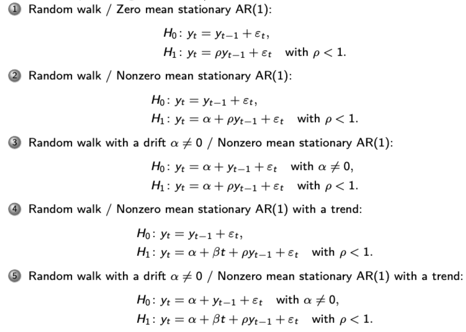
Dickey Fuller and ADF tests (including consequences of under and overspecification

Tests for non-stationarity in the process. Different Dickey-Fuller tests shown. Choose accordingly. Estimate parameters via OLS then use t-test against relevant DF critical values to see this (if significant then reject the null of a unit root)

Use the ADF test if you believe there is autocorrelation in the errors of your OLS estimation. Add lags of the differenced term to the regression. Critical values are the same as before.

Cointegration and Error Correction Mechanisms

Cointegration: the property of a collection of I(1) processes that yield an I(0) linear combination. The coefficients on this linear combination are the cointegration vector.

Error Correction Mechanisms: Show short term adjustment dynamics of cointegrated variables, ensuring that deviations from their long-run equilibrium are corrected over time. Often interpreted via economic theory (see t-bill example in slides, great ratio example in problem set)

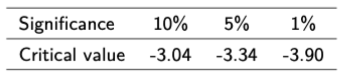
Engel Granger procedure for testing for cointegration

Regress on variable on the variable that you believe it is cointegrated with, then compute an ADF statistic on the residuals of this regression. In this case you have to use specia Engle Granger critical values. In particular, reject the null of no cointegration if t is less than the pictured crit values.

Additionally, this can be used to estimate the coefficients in the cointegrating vector, which is useful when used in error correction models.

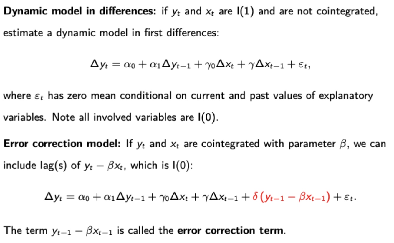
Dynamic models in differences and Error Correction Models

Different models for short run dynamics. Note that the inclusion of the Error Correction term (which is warranted when the variables are cointegrated because both sides of the equation would still be stationary) allows for a better capture of how short run deviations revert back to long run EQ.

Working out impulse response from a VAR(p) process

Convert to VAR(1) → convert to MA(inf) as shown → interpret the upper left m x m block of your coefficient matrix to get the impulse response function, remembering the exponent to get the requisite number of lags.

How to test for whether an estimator is consistent

If the asymptotic variance of the estimator approaches 0 as the sample size tends to infinity, the estimator is consistent.

ADF test

Run the regression as shown before (see PS6 answers for funky way of dealing with extra lags even though you likely won’t need to do this extra maths) then compare to DF critical values, ensuring you are using the right critical values (i.e. with / without intercept / trend). When doing this in the exam, test it over both 5% and 1% significance levels.

Changing models into their error correction form

Transform into error correction form by isolating a cointegration relationship, and then first differencing / manipulating other terms to ensure that every term on either side of the equation is stationary.

Deriving a likelihood / log likelihood function

The product of the value of the joint density at every observation of x and y with a given parameter. Log likelihood is just the log of this (so sum of the log joint density functions at every observation)

Formula for joint density f(y(i),x(i); theta)

Conditional density f(y(i); theta | x(i))* marginal density f(x(i); theta) (extension - put this in vector / matrix form)

Impact of marginal density on MLE

Assume that the marginal density doesn’t depend on the parameter of interest, so it can be ignored for likelihood maximisation.

If the marginal density does depend on the parameter, you can still estimate the parameter with MLE, but the conditional ML estimator would obviously be less efficient than the unconditional one that utilises information about the parameter from the marginal distribution of x.

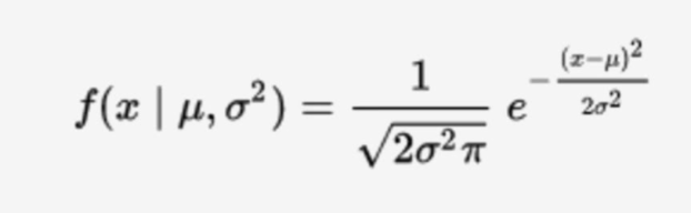
Gaussian pdf

Process for MLE estimate for a standard regression model with normal errors (remember two parameters of interest)

Identify conditional density of Y|X (normal since errors are normal), then derive the log likelihood function. Maximise log likelihood with respect to beta first, which should give the same estimator as OLS (because you are essentially minimising the residual sum of squares). Then take the FOC wrt the variance term, noting that the ML estimator for the variance is biased.

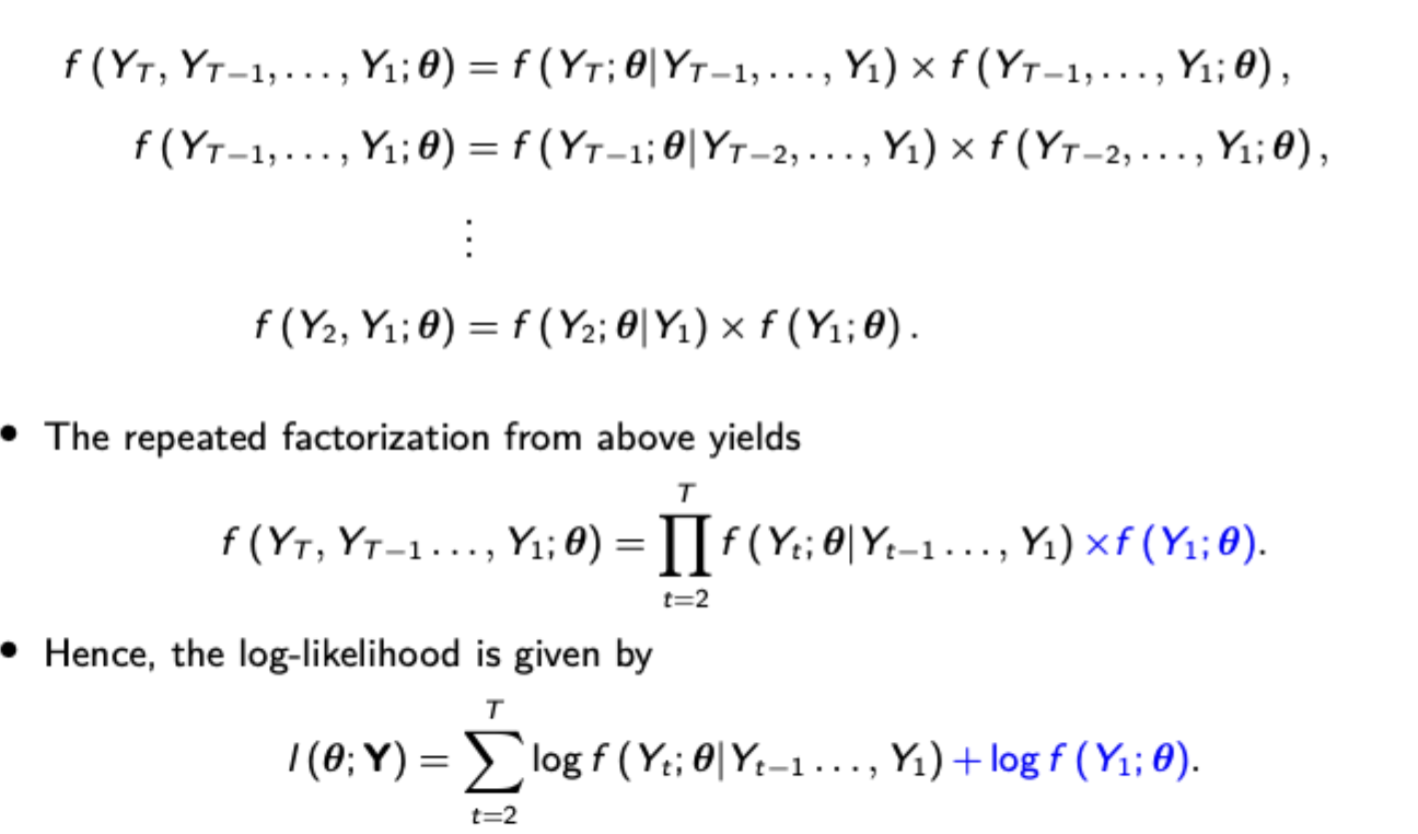
Finding a conditional density function for the dependent variable in time series data (not i.i.d.)

Use repeated factorisation, and remember the unconditional distribution of the initial value (normal with 0 mean and same variance as in AR(1) covered in time series, but needs to have its likelihood derived as well.

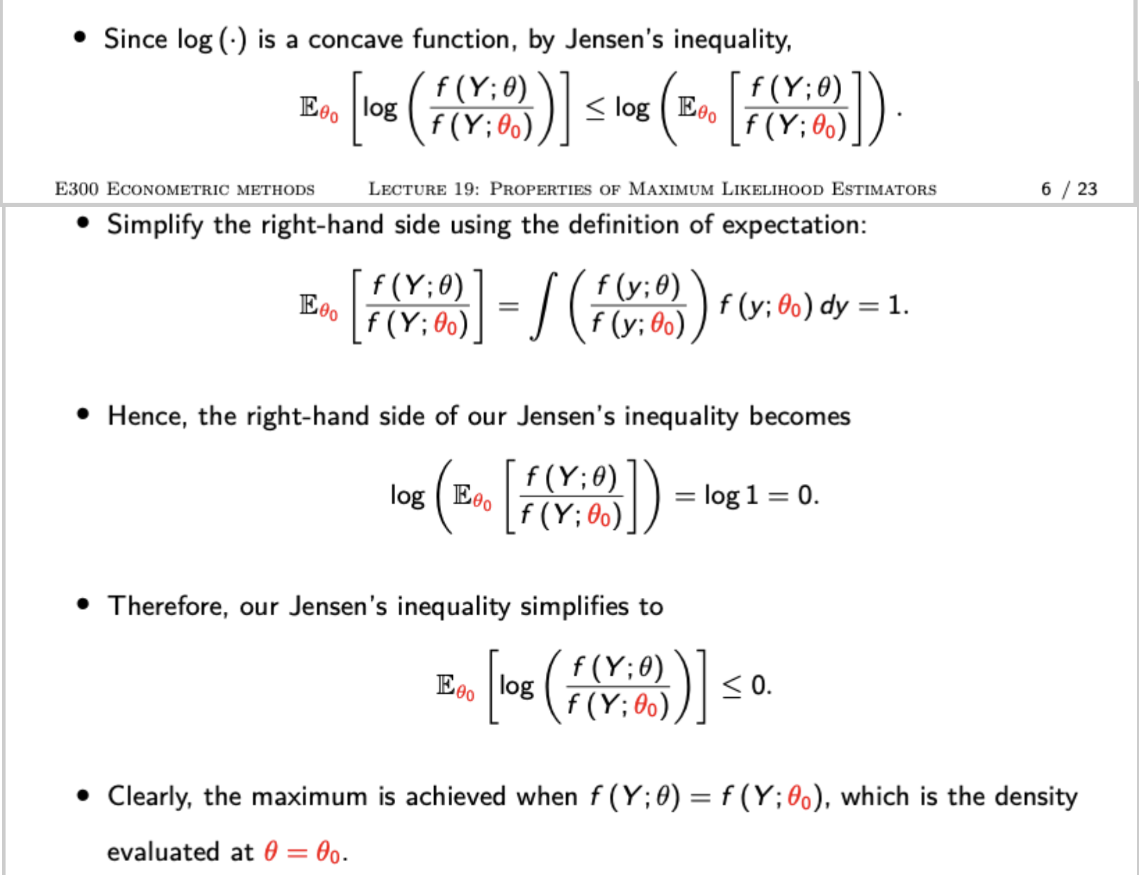
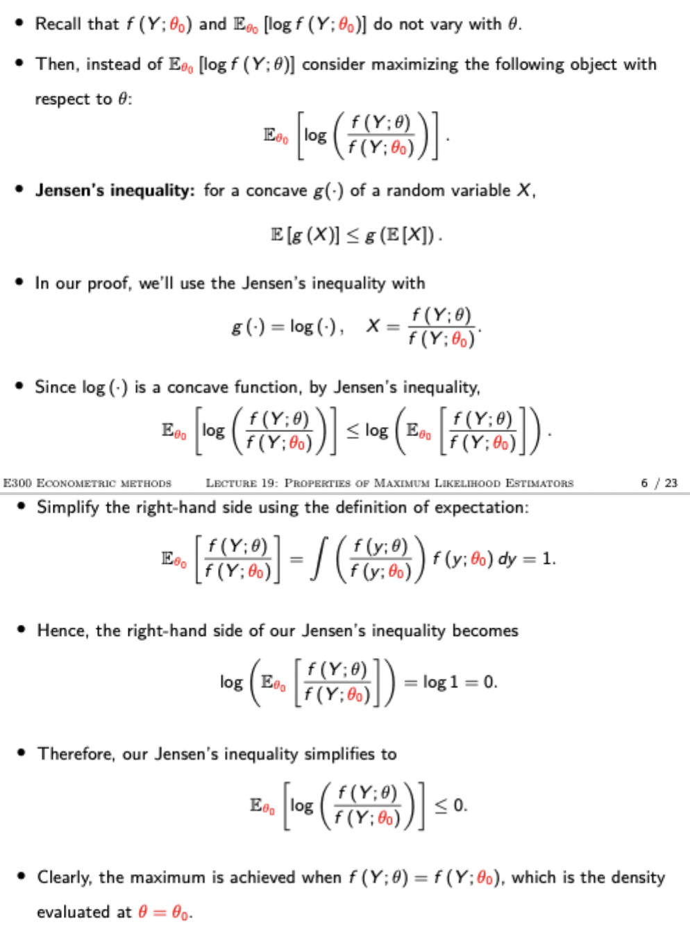
Process to show consistency of the ML estimator

Derive the likelihood function, noting that your result will be the same if you maximise your conditional likelihood function - the likelihood function of the true parameter value. Divide both sides by n and use LLN to get the expectation of your two likelihood functions over the true density. Then use Jensen’s inequality to show that your expression of the two expected log likelihoods must be less than or equal to 0 (pictured), which shows that the maximum must be achieved when your estimated parameter equals the true parameter.

Score function + individual score

Score function: partial derivative of the log likelihood function

Individual score: partial derivative of the log density

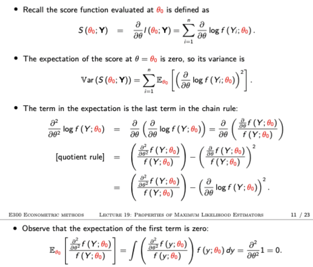
Proof that the expected value of the score function at the true parameter is 0

Fisher information

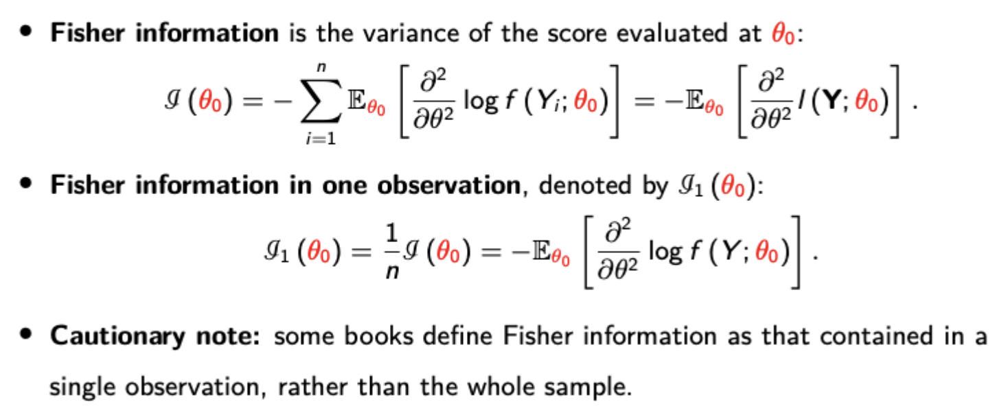
Variance of the score function at the true parameter, formula pictured.

Derivation of Fisher information and information equality.

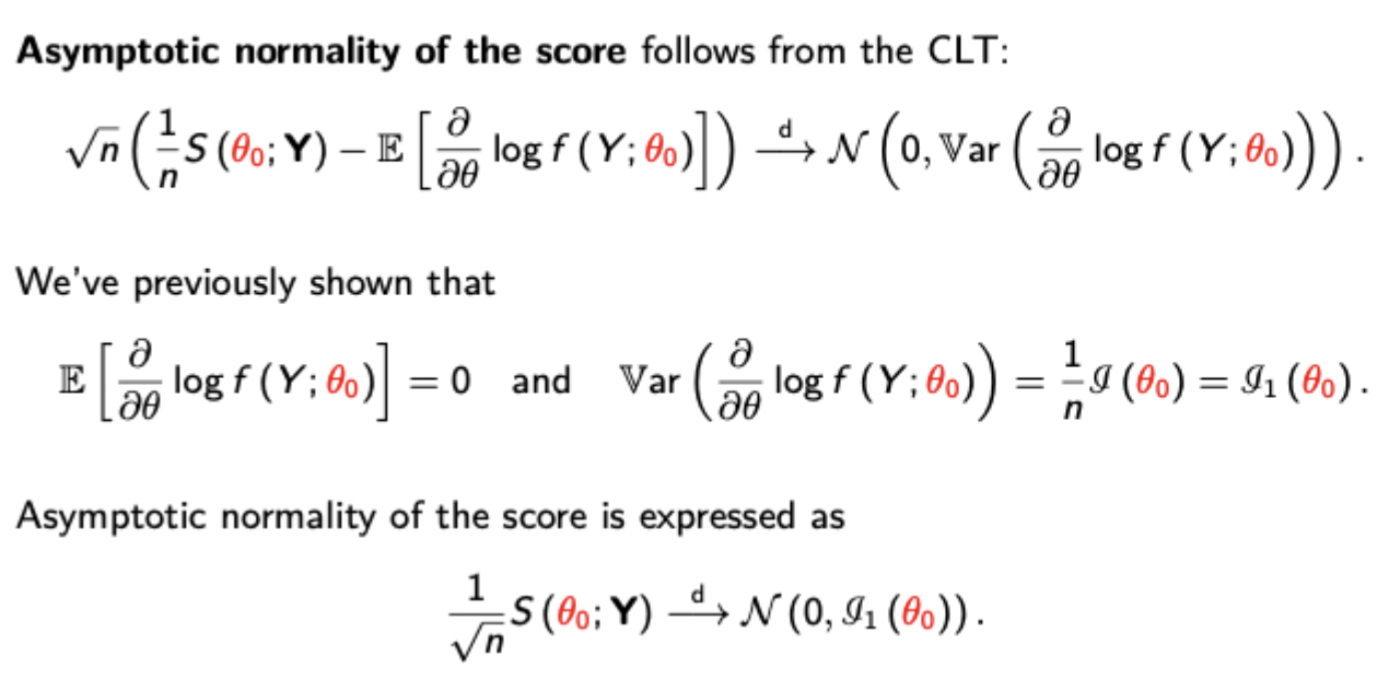
Asymptotic distribution of the score function

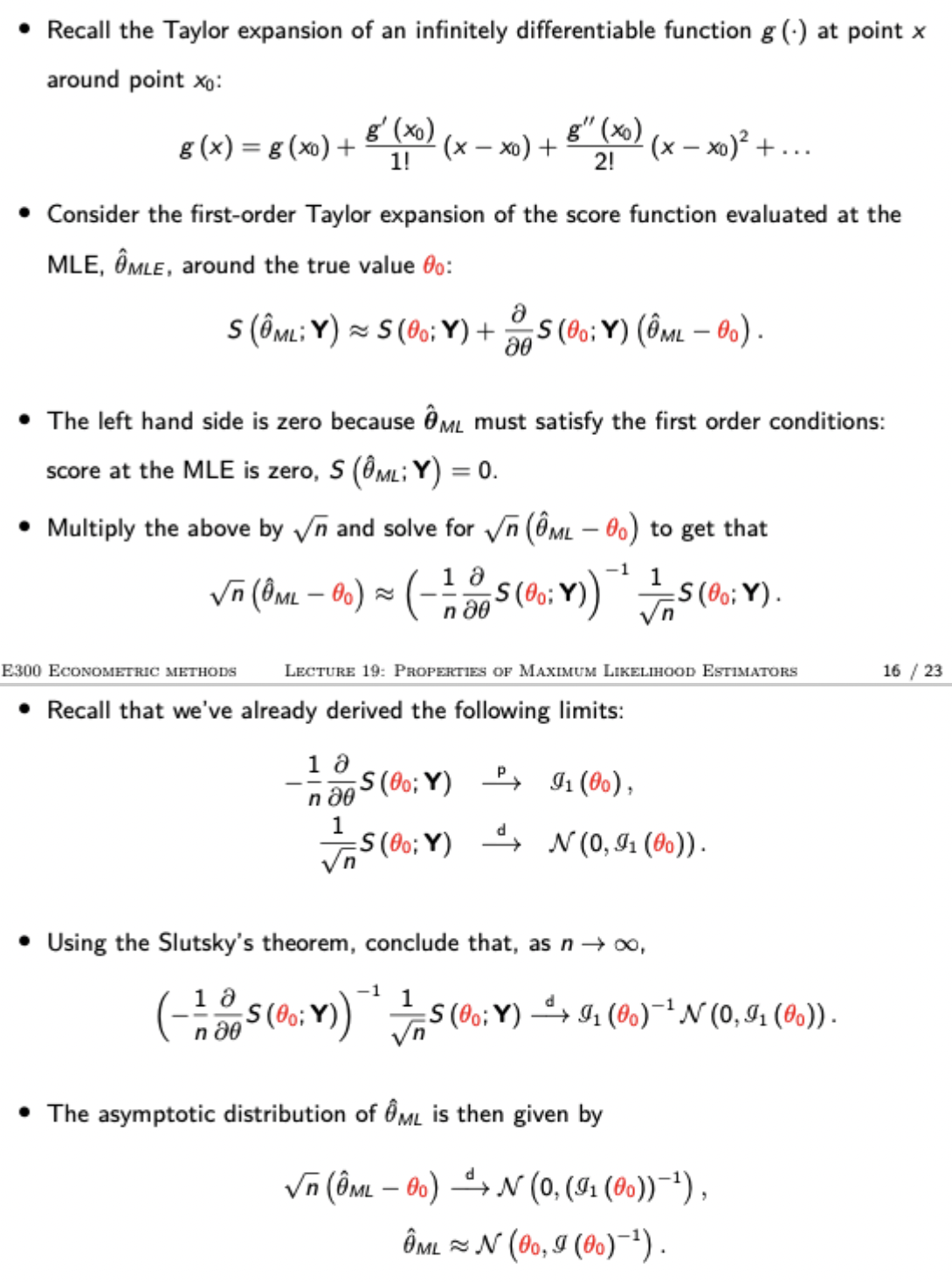
Use of Taylor approximation of the score function evaluated at the ML estimate to show that the ML estimator is asymptotically normal + asymptotic distribution of MLE

Cramer-Rao Lower Bound

The lowest possible variance for an unbiased estimator, equal to the reciprocal of the fisher information over the whole sample. Since this is the asymptotic variance of the ML estimator, it shows that MLE is asymptotically efficient (since it is asymptotically unbiased and achieves the C-R lower bound)

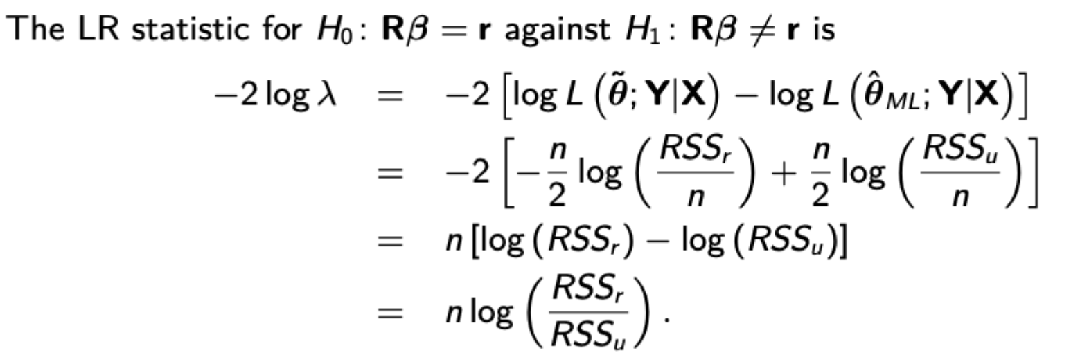
Likelihood ratio test formula + procedure (all tests have m restrictions)

Likelihood ratio lambda is the ratio of maximum likelihood under the restriction to maximum likelihood without the restriction.

The LR statistic is -2*log(lambda) and has chi squared distribution with m degrees of freedom.

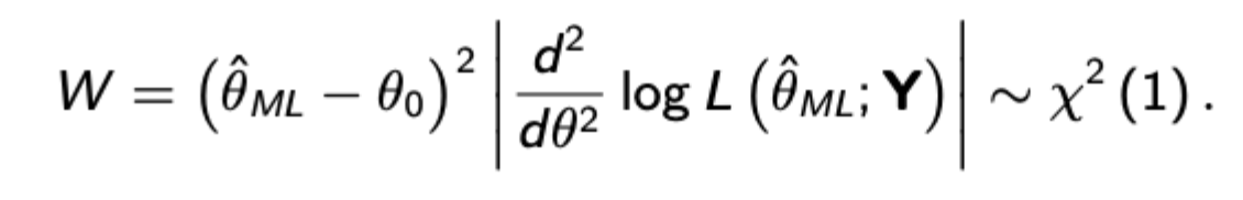
Wald test formula + procedure

Uses the absolute value of the second derivative of the log likelihood function and has a chi squared distribution with 1 degree of freedom. Proof uses a second order Taylor approximation for the restricted log likelihood around the ML estimate.

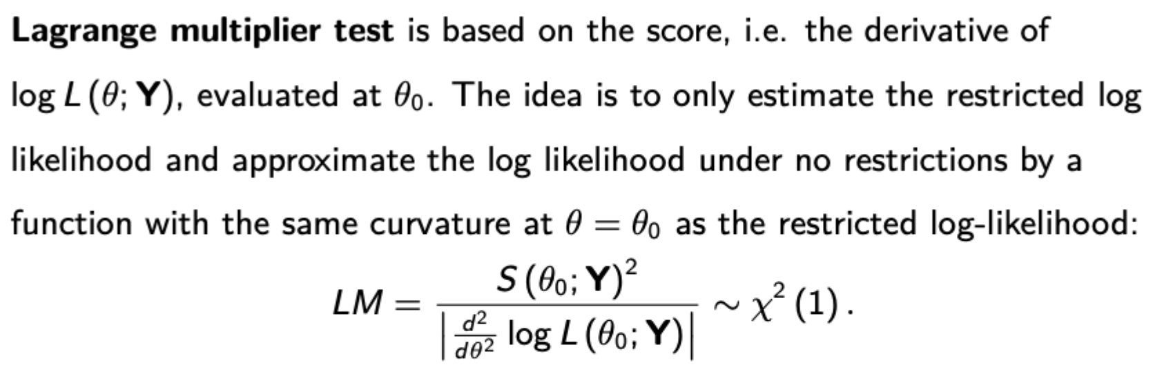
LM test formula + procedure

Remember again that this is the absolute value, not brackets

Which is the best likelihood-based test

Tests are asymptotically equivalent but may give different results in finite samples

LR test requires both restricted and unrestricted ML estimates, so may be more computationally demanding

W and LM tests are susceptible to reparameterisation of the model, whereas the LR test is invariant to this.

Order of likelihood to reject hypotheses: W → LR → LM (most likely to reject under the Wald test.

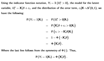
Probit Derivation (Latent Variable model)

Probit Partial Effects

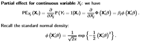
(Remember it is different for discrete variables, just find the difference between the probit function with the discrete variable and without)

Delta Method

Derives the asymptotic distribution of an RV when the RV is a differentiable function of an asymptotically Gaussian RV where sqrt(n)[X-/theta] has a distributional limit of N(0,/sigma²)

Bernoulli PDF

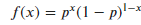
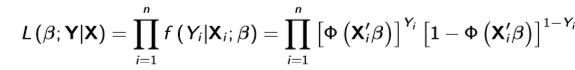
Conditional likelihood function for Probit

Applies because Y|X is a Bernoulli random variable with y either 0 or 1. The total likelihood function is this * marginal density of X, but can be ignored so long as the marginal density doesn’t depend on the parameters of interest. Even if it does, it may be better to limit attention to the conditional likelihood since misspecification of the marginal density may result in inconsistent MLE

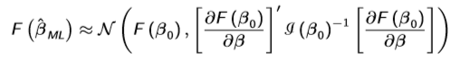
Asymptotic distribution of a differentiable nonlinear function of a parameter estimated by MLE

Works because we know that beta is asymptotically normal from MLE

Stationarity of VAR(p) as VAR(1)

When writing VAR(p) as VAR(1), (as shown), stationarity can be shown when the eigenvalues of F are less than one in absolute value (see picture for reminder of how to calculate eigenvalues)

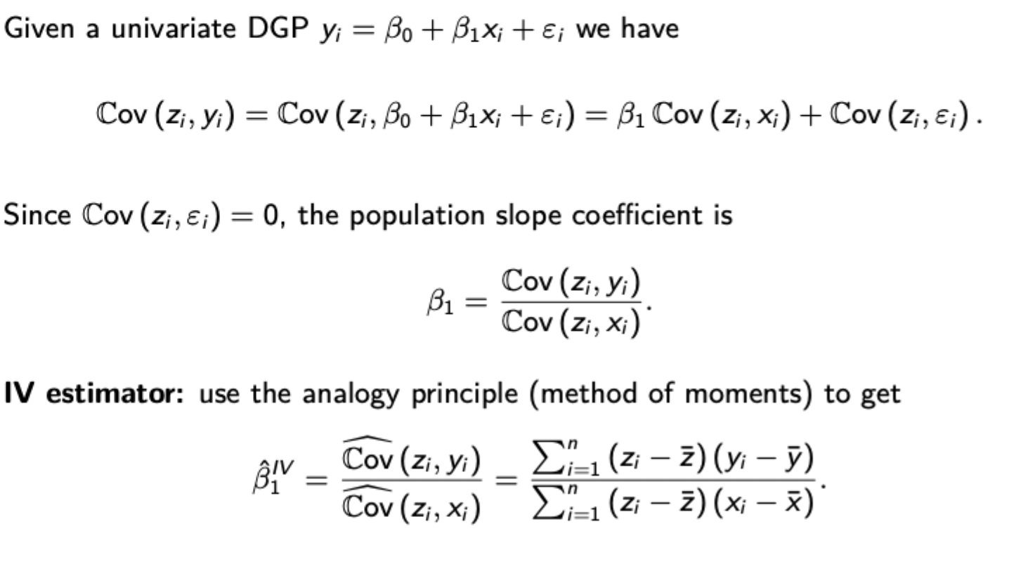
Derivation of univariate IV estimator

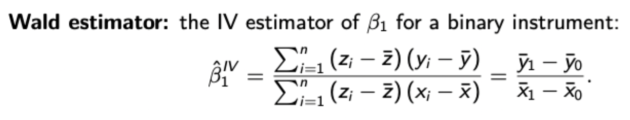
Wald estimator (with binary instrument)

Why might the IV estimator be biased in small samples (even though it is consistent)

If the instrument is weak, the denominator may become very small or even 0, hence the expected value of your estimated coefficient may not even exist for some small sampels

How to show asymptotic normality of the IV estimator

Calculating the variance of the IV estimator

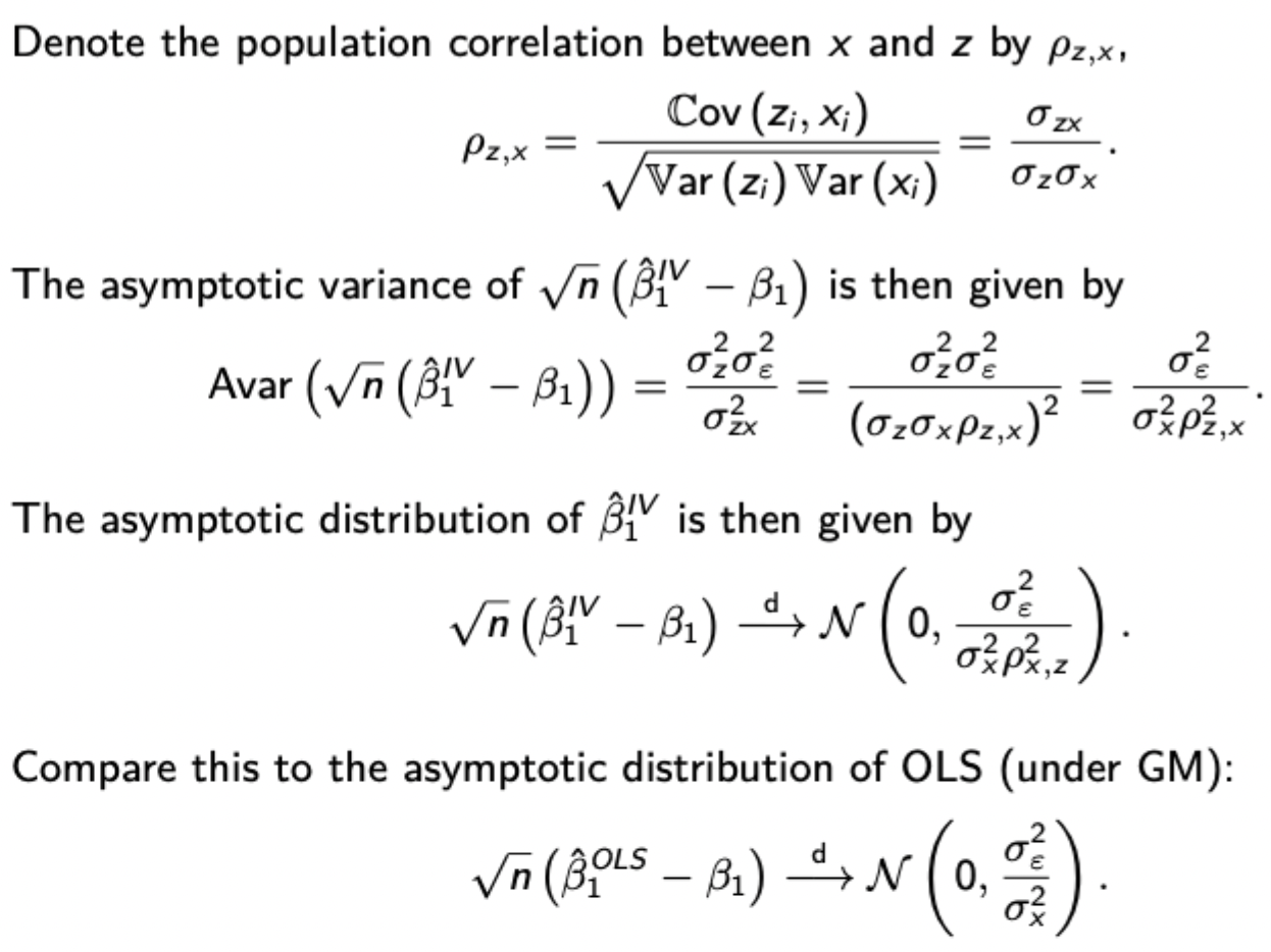
(note that the variance may be far larger than OLS if the correlation between z and x is very small)

How do weak instruments jeopardise consistency of the IV estimator?

How do weak instruments exacerbate the effects of instrument endogeneity

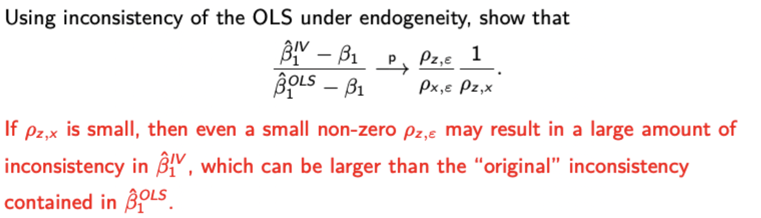
(Note that if this is pronounced, enough, the IV estimator may have greater inconsistency than the endogenous OLS estimate)

Derive the IV estimator with additional exogenous explanatory variables

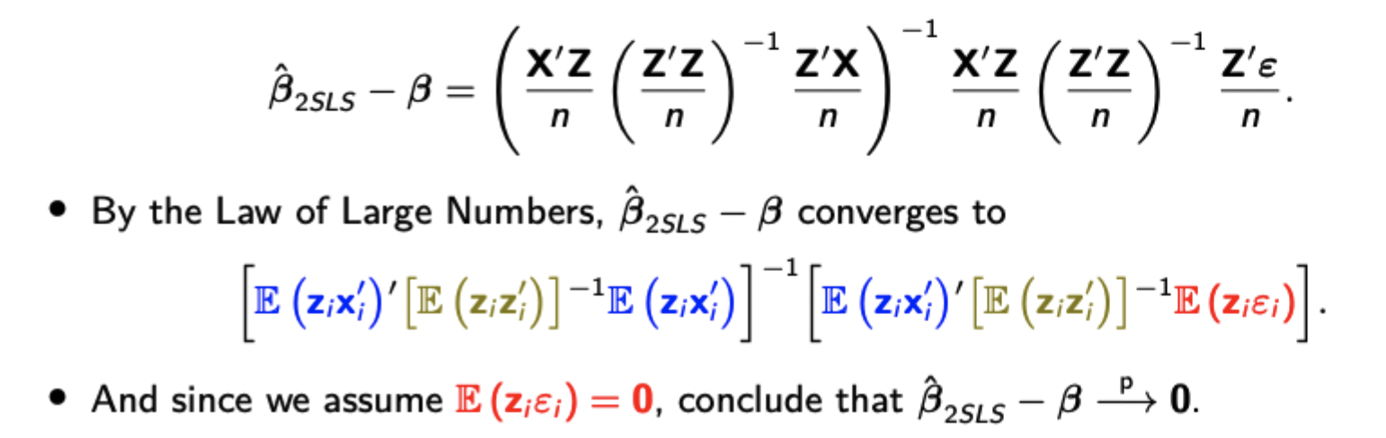
Derivation of the 2SLS estimator

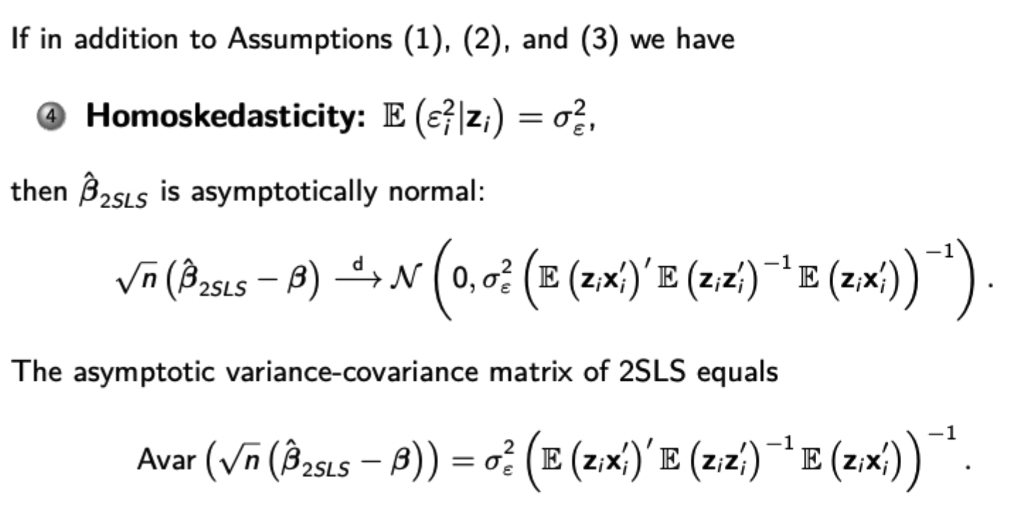
Show consistency of the 2SLS estimator and asymptotic normality

What is the variance estimate for the 2SLS estimator?

Testing for endogeneity

Regress your suspected endogenous variable on your set of instruments, then regress y on all explanatory variables and the residuals from your initial regression (coefficients should be unaffected here by FWL theorem). If the coefficient on the residuals is significant (>0) then the variable is endogenous. If not, it is exogenous and 2SLS is unnecessary and costly.

Rule of thumb value for finding weak instruments

If the F stat for coefficients in the first stage of the 2SLS regression is less than 10, then you have weak instruments and should either find new ones or remove the weakest ones to see if this strengthens your F stat.

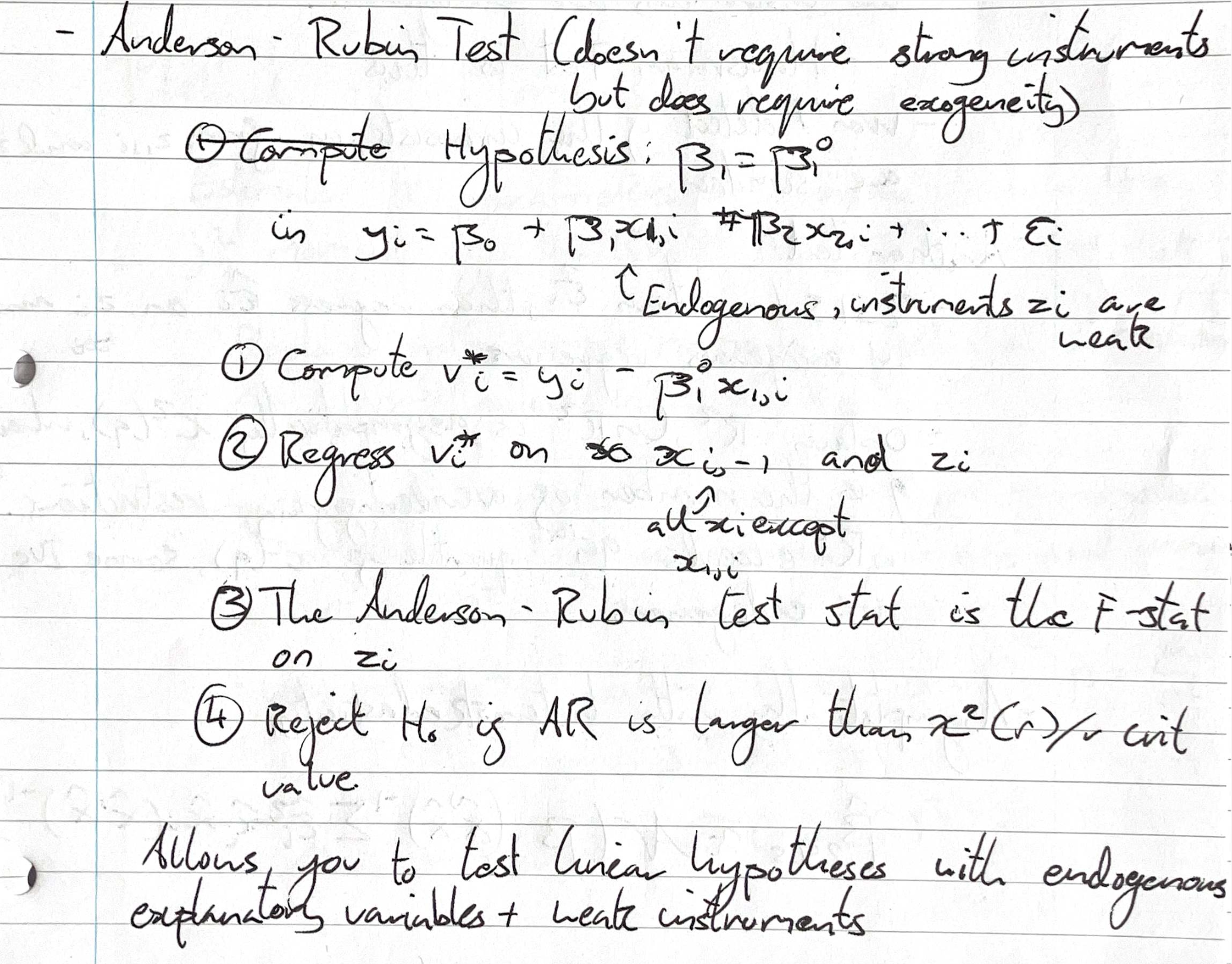
Anderson Rubin Test for linear hypotheses when you have weak (but exogenous) instruments

Hausman test (overidentifying restrictions test) for instrument endogeneity

(Example of 2 instruments for 1 endogenous variable)

Do 2SLS twice: once with one of the instruments, once with the other. If the difference between the estimates is large, then one or both of the instruments is endogenous (note that if the inconsistency from both instruments is similar, then the Hausman test won’t detect it)

Alternative test for instrument endogeneity

Use 2SLS to obtain estimated residuals (note these are the residuals from your fitted regression, not your second stage regression). Then regress the residuals on all exogenous regressors and all instruments. Obtain the R², where nR² is asymptotically chi-squared distributed with the number of overidentifying restrictions as its degrees of freedom. If nR² exceeds the 95th quantile of this, then some IVs are endogenous.

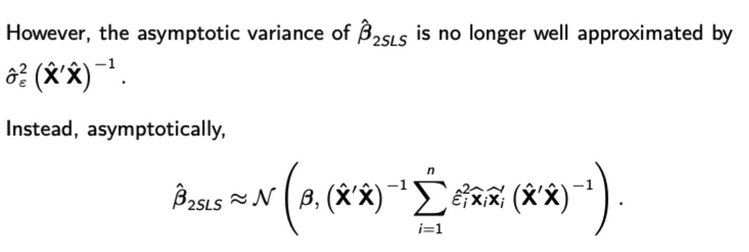
Asymptotic distribution of the 2SLS estimator with heteroskedasticity

Conditions for asymptotic inference to hold for 2SLS with time series data

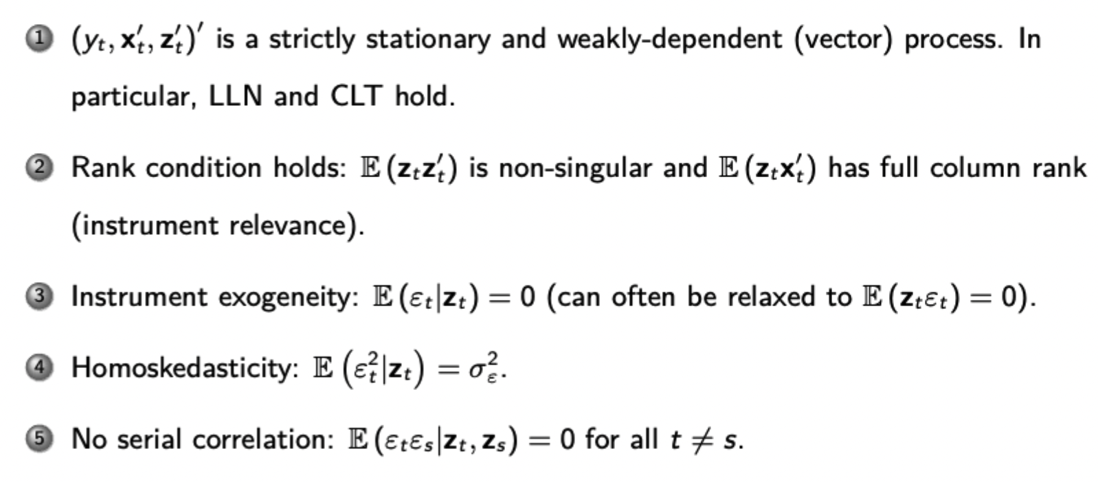
Conditions for finite sample inference to hold with any data

Must satisfy the Gauss-Markov assumptions

How do Method of Moments estimators work

Estimate k parameters using given expressions for the k moments of your random variable (therefore getting k expressions for k parameters) and then replacing these moments with the sample moments to get the estimate.

Formal definition of the GMM estimator

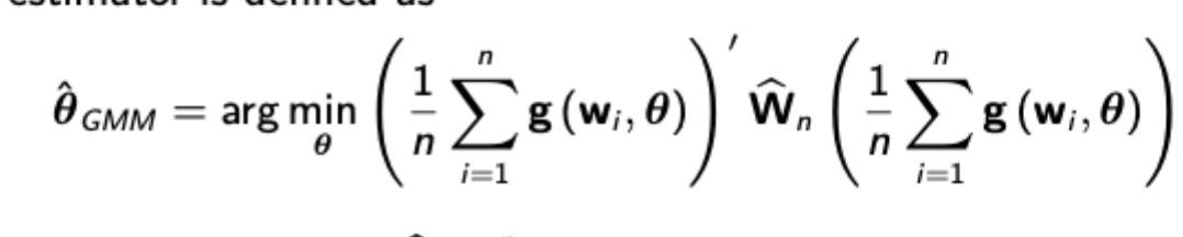
Uses a weighting matrix to combine multiple moment conditions (esimated via sample moments) into a quadratic form. This weighting matrix is chosen optimally so as to minimise the asymptotic variance of the estimator.

What is the optimal weighting matrix for GMM

It is the reciprocal of the variance expression (which you will likely have to estimate, but may be given)

Show how optimal GMM under homoskedasticity with an endogenous variable is 2SLS

For any vector of regressors A, when is the Pa*X1 = X1? (Pa is the projection matrix of A)

This is true when A contains a column that is linearly dependent with X1 (i.e. X1, or some form of linear transformation of X1, is a column of A)

Meaning of an iid sample of (y,x)

Each pair of (yi, xi) is independent with identical distribution. DOES NOT MEAN that y is independent of x, so you cannot use this to assume conditional / unconditional independence / 0 covariance between errors and regressors.

Points to evaluate an ADF specification

• Even if the ADF specification includes additional lags, it assumes that shocks are all serially uncorrelated which may be very demanding

• It may not include sufficient consideration for any potential deterministic breaks which you might be able to see in the data.

Tests for serial correlation / heteroskedasticity

• Heteroskedasticity:

  • Breusch-Pagan: Regress squared residuals linearly on all explanatory variables and compare F statistic to critical values F(k,n-k-1) dist the asymptotic transformation to chi squared (almost identical for large n)

  • White: Regress squared residuals on continually increasing powers of predicted y (which is just a function of explanatory variables) then compute F statistic and compare against critical values

• Serial Correlation:

  • Breusch-Godfrey: Compute LM statistic (T-q)*R² using R² from regression of residuals on explanatory variables and lagged residuals (q restrictions). Use chi-squared critical values with q d.f.

  • F-test from regression of residuals on explanatory variables and lagged residuals (Testing hypothesis that the coefficients on the residual lags are all 0)

What to do if there is heteroskedasticity / serial correlation in errors

• Find a better model

• Use heteroskedasticity robust / HAC standard errors

• Use GLS / FGLS (can do it in different ways if needs be)

F Statistic - Both formulas

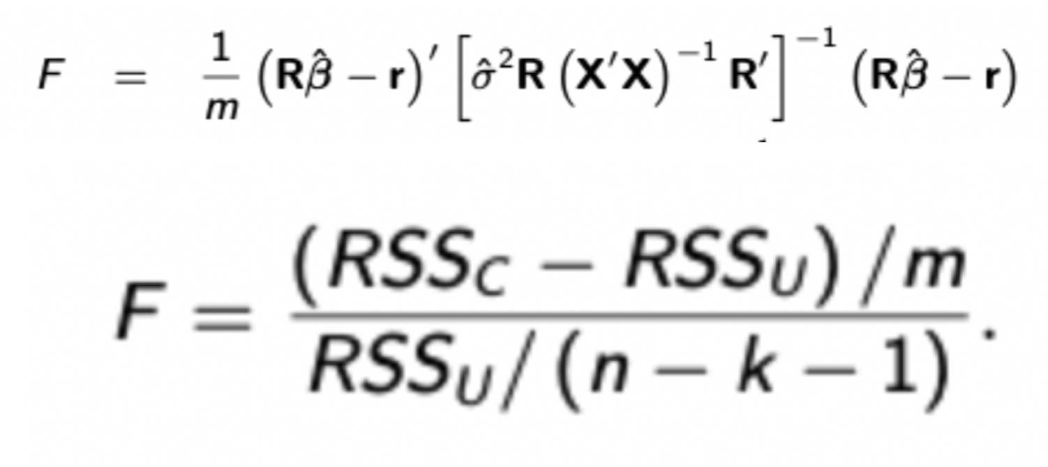
Also recall derivation for the first formula

F and t distributions

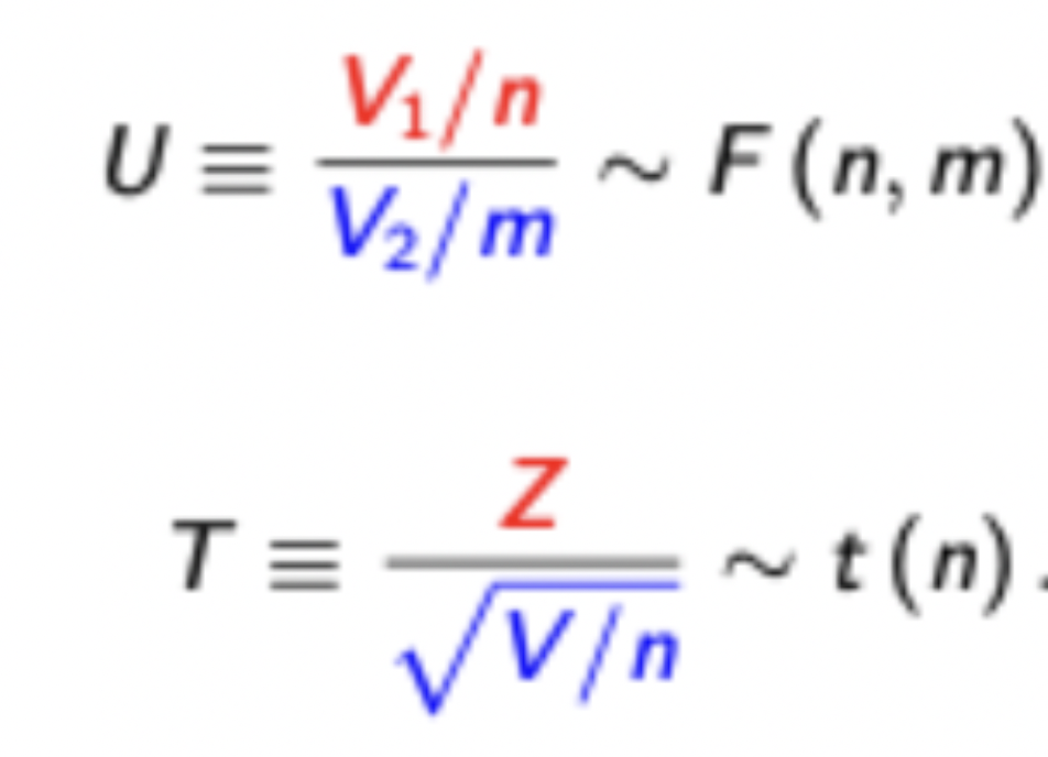
Use t when there is only one restrictions. It is the ratio of a standard normal RV (i.e. your hypothesis) on top of the square root of a chi-squared RV (i.e. the variance estimator) normalised by its degrees of freedom.

Difference in handling endogeneity between the causal and ‘best linear predictor’ interpretations of OLS

• The causal interpretation sees OLS as estimating the causal mechanism between x and y, making the error term ‘all other factors’. Endogeneity is thus likely and will greatly harm the accuracy of your estimated causal effect

• The BLP interpretation gives the OLS estimate as the just the best way to fit x to y in a linear fashion. The error term is thus just the errors of the observed y given x, and is not a function of all other factors like in causal interpretation. Therefore endogeneity is not a problem, even though the coefficient would be biased for causal interpretation. The assumption E(xe) = 0 is essentially free.

Dynamic completeness as a sufficient condition for the no serial correlation assumption in assyptotic time series OLS

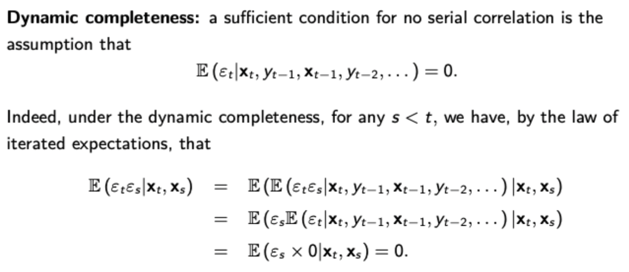
As opposed to assuming no serial correlation, which implies that the model explains all of y’s dynamics

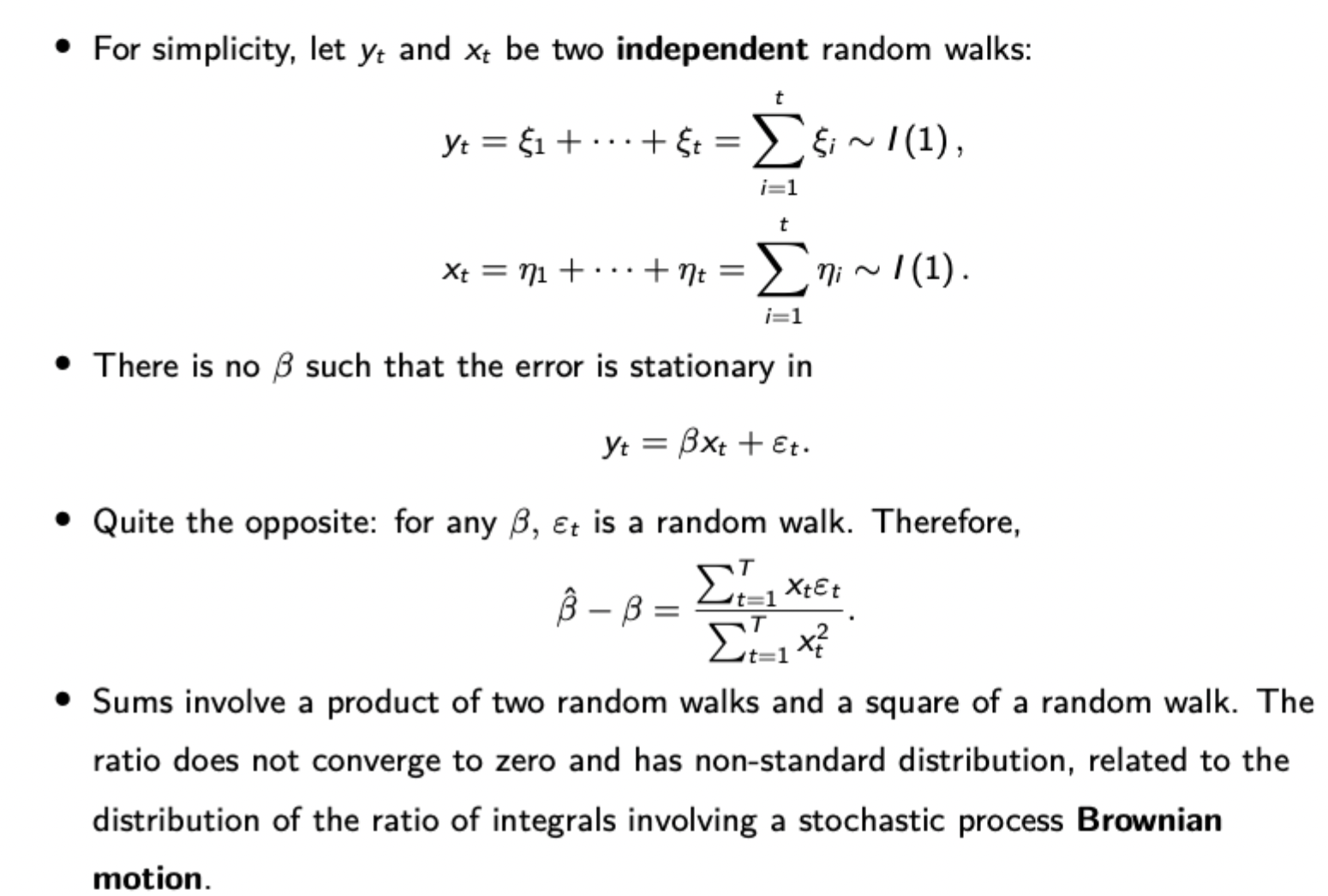
Source of the spurious regression problem