Producer and Consumer Behavior

income changes

pure income effect

price changes

income and substitution effects

normal goods

higher income = more consumption

inferior goods

higher income = less consumption

income effect

change in consumer choices resulting from change in income and purchasing power, holding price constant

income expansion path (IEP)

curve that connects consumer’s optimal bundles at each income level

IEP positive slope

both goods normal

IEP negative slope

1 good inferior

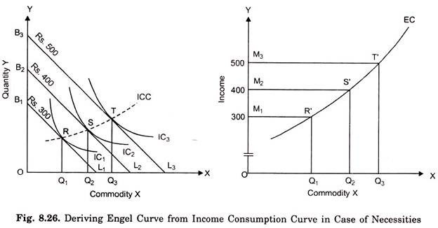
engel curve

shows relationship between quantity consumed and income; goods can transition from normal to inferior

positive engel slope

good is normal at that income level

negative engel slope

good is inferior at income level

deriving a demand curve

1. define relationship 

2. change one price, observe changes in consumer choices 

3. observed price = maximum willingness to pay for the last unit consumed

substitution effect

change in consumption resulting from a change in relative price of two goods

income effect 

change in consumption resulting from a change in purchasing power of income 

inferior good changes

• increase in purchasing power = decrease consumption

• decrease purchasing power = increase consumption

normal good changes

• increase in purchasing power = increase consumption

• decrease purchasing power = decrease consumption 

total effect

substitution effect + income effect

isolating substitution effect

determine bundle of goods that would have been chosen at new price while maintaining utility experience before change in price; find where the new indifference curve would be parallel to new price/budget 

isolating income effect

change in Q_D due to change in purchasing power after change in price (whatever is left after substitution effect)

purchasing power change on graph

BC1 to BC2

Income effect on graph

A’ to B

Substitution effect on graph

A to A’

market demand 

horizontal sum of individuals’ demand curves

market quantity

sum of individuals’ quantity demanded at each price

production

process by which firms use inputs to create outputs

final goods 

goods bought by consumers (bread) 

intermediate goods

goods used to produce another good (wheat)

production function

mathematical relationship between inputs and how much output is made

production function equation

Q = K^aL^(1-a) ; a<=1

capital (K)

building, equipment

labor (L)

human resources 

assumptions of production

1. firm produces 1 good 

2. firm has already chosen the product to produce 

3. only two inputs: capital and labor 

4. capital fixed in short run, adjustable in long run 

5. more inputs = more outputs 

6. inputs are characterized by diminishing returns 

7. firm can buy as much capital and labor as it wants to borrow 

marginal product (MP)

additional unit of output using additional input (holding use of other input constant)

Marginal Product of Labor (MP_L)

aQ(L,K)/aL 

Marginal Product of Capital (MP_K)

aQ(L,K)/aK

diminishing MPL

decline in output rate, not level; tends to happen in short run; doesn’t always have to diminish, only eventually

isoquant

“same quantity”; combinations of capital and labor that yield the same output

characteristics of isoquants

• further from origin = higher output 

• can’t intersect 

• convex to origin

Slope of Isoquant

Marginal Rate of Technical Substitution

Marginal Rate of Technical Substitution

MRTS_K,L= MP_L / MP_k

isocost

“same cost”; all input bundles that cost the same

W

wage; expense of labor

R

rent; cost of capital

Cost Equation

W*L + R*K 

slope of cost

-W/R

cost minimizing condition

MP_L / MP_k = W/R

Marginal Product Per Dollar Labor

MP_L / W 

Marginal Product Per Dollar Capital

MP_K / R 

Returns to Scale

change in output when all inputs are increased in the same proportion

constant returns to scale

production increases proportionally to inputs

increasing returns to scale

changing inputs changes the outputs more than proportionally

decreasing returns to scale

changing inputs by the same proportion changes the output less than proportionally

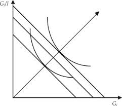
firm expansion path 

illustrates how the optimal mix of inputs varies with total output 

total cost curve 

firm’s cost of producing particular quantities 

accounting cost 

direct costs of operating a business

economic costs

accounting cost + opportunity cost

accounting profit

firm’s total revenue - accounting cost

economic profit

total revenue - economic cost

fixed cost 

cost of fixed inputs, independent of output 

variable cost 

cost of inputs that vary with output 

total cost

fixed cost + variable cost

average total cost

TC/Q

average fixed cost

FC/Q

Average variable cost

VC/Q

AFC curve

always declining

AVC & ATC Curves

U-shaped

marginal cost

additional cost of producing additional unit of output

MC

dTC/dQ (FULL DERIVATIVE)

MC < ATC 

cost of producing one more unit is less than average cost; average cost falls with unit 

MC > ATC

cost of producing one more unit is more than average cost; average cost rises with unit 

MC = ATC

average is at minimum

economies of scale

cost rises more slowly than production

constant economies of scale

cost rises at same rate as production

diseconomies of scale

cost rises more quickly than production