Macro Ch 11-16 Textbook
5.0(1)
Studied by 7 peopleCard Sorting
1/90
There's no tags or description
Looks like no tags are added yet.
Last updated 7:24 PM on 4/23/23
Name | Mastery | Learn | Test | Matching | Spaced | Call with Kai |
|---|
No analytics yet
Send a link to your students to track their progress
91 Terms
1
New cards
Classical Theory of Inflation
* Quantity theory of money
* Most economists today rely on this theory to explain the long-run determinants of the price level and the inflation rate.
* Most economists today rely on this theory to explain the long-run determinants of the price level and the inflation rate.
2
New cards
Value of Money Equation
* P is price level and measures the number of dollars needed to buy a basket of goods and services
* turn this idea around: The quantity of goods and services that can be bought with $1 equals 1/P.
* 1/P is the value of money measured in terms of goods and services.
* Ex. a cone costs $2, P=2
* 1/P, means the value of a collar is half a cone
\
*When the overall price level rises, the value of money falls*
3
New cards
Variable that affect the demand for money
* the average level of prices in the economy
* In the long run, the overall level of prices adjusts to the level at which the demand for money equals the supply (equilibirum)
* If the price level is above the equilibrium level, people will want to hold more money than the Bank of Canada has created, so the price level must fall to balance supply and demand.
* If the price level is below the equilibrium level, people will want to hold less money than the Bank of Canada has created, and the price level must rise to balance supply and demand.
4
New cards
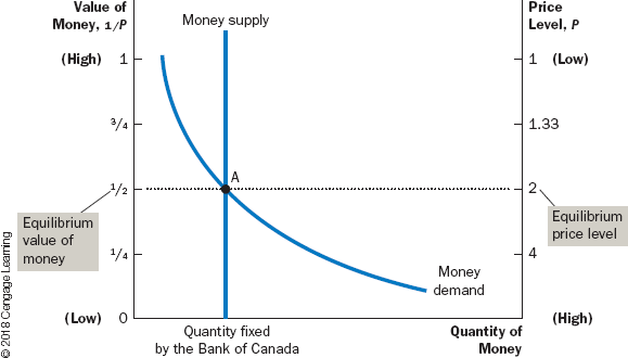
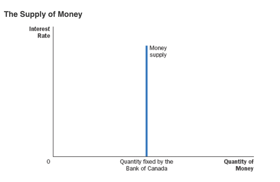
Supply and Demand Curve for Money
* Horizontal axis shows quantity of money
* Left vertical shows the value of money 1/p
* right vertical shows the price level P
* Top, low level
* Bottom, high level
* When the value of money is high (as shown near the top of the left axis), the price level is low (as shown near the top of the right axis).
* The supply curve is vertical because the Bank of Canada has fixed the quantity of money available.
* The demand curve for money is downward sloping, indicating that when the value of money is low (and the price level is high), people demand a larger quantity of it to buy goods and services.
* Equlibirum determines the value of money and the price level
5
New cards
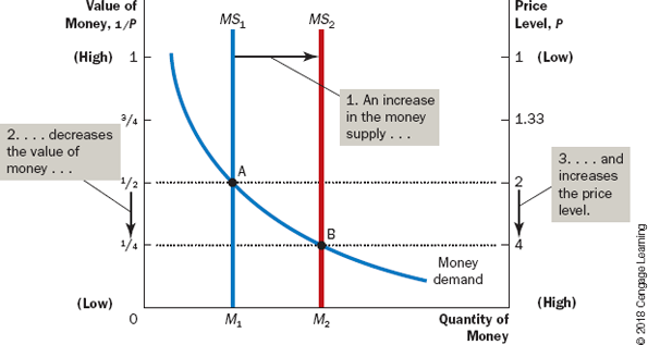
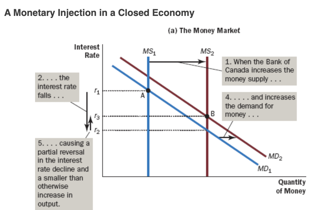
Effects of Money Injection
* Money injection shifts the supply curve to the right (from MS1 to MS2)
* This move equilibrium from point A to B
* Value of money (shown on the right) decreases from 2 to 4
* In other words, when an increase in the money supply makes dollars more plentiful, the result is an increase in the price level that makes each dollar less valuable.
* This move equilibrium from point A to B
* Value of money (shown on the right) decreases from 2 to 4
* In other words, when an increase in the money supply makes dollars more plentiful, the result is an increase in the price level that makes each dollar less valuable.
6
New cards
Quantity Theory of Money
* This explanation of how the price level is determined and why it might change over time
* According to the quantity theory, the quantity of money available in the economy determines the value of money, and growth in the quantity of money is the primary cause of inflation.
* According to the quantity theory, the quantity of money available in the economy determines the value of money, and growth in the quantity of money is the primary cause of inflation.
7
New cards
Nominal variables
variables measured in monetary units.
* Ex Nominal GDP
* Ex Nominal GDP
8
New cards
real variables
variables measured in physical units.
* Ex. Real GDP
* Ex. Real GDP
9
New cards
classical dichotomy
* The seperatio of variables into real and nominal
10
New cards
Monetary Neutrality
* This irrelevance of monetary changes for real variables in the long run
* the proposition that changes in the money supply do not affect real variables
* the proposition that changes in the money supply do not affect real variables
11
New cards
Classical Theory on Long Run Economy
* Over the course of a decade, for instance, monetary changes have important effects on nominal variables (such as the price level) but only negligible effects on real variables (such as real GDP).
* Monetary Neutrality is a good description of how the world works in terms of long ryn changes in the economy
* Monetary Neutrality is a good description of how the world works in terms of long ryn changes in the economy
12
New cards
Velocity of Money.
* The rate at which money changes hands
* The speed at which the typical dollar travels around the economy from wallet to wallet.
* The speed at which the typical dollar travels around the economy from wallet to wallet.
13
New cards
Calculating Velocity of Money
V=(PxY)/M
* V: Velocity
* P: Price Level (GDP Deflator)
* Y: Quantity of output (Real GDP)
* M: Quantity of Money
* V: Velocity
* P: Price Level (GDP Deflator)
* Y: Quantity of output (Real GDP)
* M: Quantity of Money
14
New cards
Quantity Equation
MxV=PxY
* Rearranged velocity equation
* V: Velocity
* P: Price Level (GDP Deflator)
* Y: Quantity of output (Real GDP)
* M: Quantity of Money
Shows that an increase in the quantity of money in an economy must be reflected in one of the other three variables:
* The price level must rise,
* the quantity of output must rise,
* the velocity of money must fall.
15
New cards
Equilibirum Price Level and Inflation Explained
* The velocity of money is relatively stable over time.
* Because velocity is stable, when the quantity of money (M) changes, it causes proportionate changes in the nominal value of output (P×Y).
* The economy’s output of goods and services (Y) is primarily determined by factor supplies (labour, physical capital, human capital, and natural resources) and the available production technology. In particular, because money is neutral, money does not affect output.
* With output (Y) determined by factor supplies and technology, when the central bank alters the money supply (M) and induces proportional changes in the nominal value of output (P×Y) , these changes are reflected in changes in the price level (P).
* Therefore, when the central bank increases the money supply rapidly, the result is a high rate of inflation.
16
New cards
inflation tax
the revenue the government raises by creating money
* When the government prints money, the price level rises, and the dollars in your pocket are less valuable.
* The inflation ends when the government institutes fiscal reforms—such as cuts in government spending—that eliminate the need for the inflation tax.
* When the government prints money, the price level rises, and the dollars in your pocket are less valuable.
* The inflation ends when the government institutes fiscal reforms—such as cuts in government spending—that eliminate the need for the inflation tax.
17
New cards
Real and Nominal Interest Rate Equation
Real = Nominal Interest Rate- Inflation Rate
Nominal= Real Interest Rate + Inflation rate
Nominal= Real Interest Rate + Inflation rate
18
New cards
Fisher Effect
The one-for-one adjustment of the nominal interest rate to the inflation rate
* When the Bank of Canada increases the rate of money growth, the result is both a higher inflation rate and a higher nominal interest rate.
* Does not hold in the short run because inflation is unanticipated
* When the Bank of Canada increases the rate of money growth, the result is both a higher inflation rate and a higher nominal interest rate.
* Does not hold in the short run because inflation is unanticipated
19
New cards
The Inflation Fallacy
Believing that a rise in prices (inflation) means an equal loss in purchasing power
20
New cards
Costs of Inflation
* Shoeleather Costs
* Menu Costs
* Relative-price Variability and the Misallocation of Resources
* Inflation-Induced tax Distortions
* Confusion and Inconvenience
* Arbitrary Redistributions of Wealth
* Menu Costs
* Relative-price Variability and the Misallocation of Resources
* Inflation-Induced tax Distortions
* Confusion and Inconvenience
* Arbitrary Redistributions of Wealth
21
New cards
Shoeleather Costs
The cost of reducing your money holdings
* The cost of reducing your money holdings is the time and convenience you must sacrifice to keep less money on hand than you would if there were no inflation.
* The resources wasted when inflation encourages people to reduce their money holdings
* the cost of time and effort that people spend trying to counteract the effects of inflation,
22
New cards
Menu Costs
* The cost of price adjustments
* Firms change prices infrequently because there are costs of changing prices
* Include the cost of deciding on new prices, the cost of printing new price lists and catalogues, the cost of sending these new price lists and catalogues to dealers and customers, the cost of advertising the new prices, and even the cost of dealing with customer annoyance over price changes.
* The more inflation rises, the more firms must change their prices which is costly
23
New cards
Relative-Price Variability and the Misallocation of Resources
* Because prices change only once in a while, inflation causes relative prices to vary more than they otherwise would.
* market economies rely on relative prices to allocate scarce resources.
* Consumers decide what to buy by comparing the quality and prices of various goods and services.
* When inflation distorts relative prices, consumer decisions are distorted, and markets are less able to allocate resources to their best use.
24
New cards
Inflatoin Induced Tax Distortions
* lawmakers often fail to take inflation into account when writing the tax laws; economists who have studied the issue conclude that inflation tends to raise the tax burden on income earned from savings.
* taxes already distorts buying incentives, and inflation makes this worse
* higher inflation tends to discourage people from saving
* taxes already distorts buying incentives, and inflation makes this worse
* higher inflation tends to discourage people from saving
25
New cards
Confusion and Inconvenience
* When the Bank of Canada increases the money supply and creates inflation, it erodes the real value of the unit of account.
* inflation makes investors less able to sort out successful from unsuccessful firms, which in turn impedes financial markets in their role of allocating the economy’s saving to alternative types of investment.
* inflation makes investors less able to sort out successful from unsuccessful firms, which in turn impedes financial markets in their role of allocating the economy’s saving to alternative types of investment.
26
New cards
Arbitrary Redistributions of Wealth
* Unexpected changes in prices redistribute wealth among debtors and creditors.
* Inflation is especially volatile and uncertain when the average rate of inflation is high.
* If a country pursues a high-inflation monetary policy, it will have to bear not only the costs of high expected inflation but also the arbitrary redistributions of wealth associated with unexpected inflation.
27
New cards
Friedman rule
rescription for moderate deflation
28
New cards
closed economy
an economy that does not interact with other economies.
29
New cards
open economy
an economy that interacts freely with other economies around the world
30
New cards
How an economy interacts with other economies
* Buys and sells goods and services in world product markets
* Buys and sells capital assets (ex. stocks and bonds)in world financial markets
* Buys and sells capital assets (ex. stocks and bonds)in world financial markets
31
New cards
Net Exports Equation
= Value of Country’s Exports - Value of Country’s Imports
32
New cards
Trade Balance aka Net Exports
* the value of a nation’s exports minus the value of its imports
33
New cards
Trade Surplus
When a country exports more than it imports
34
New cards
Trade Deficit
When a country imports more than it exports
35
New cards
Balanced Trade
* When Exports and Imports are equal
* Net Exports are 0
* Net Exports are 0
36
New cards
Net Capital Outflow (NCO) (aka Net Foreign Investment)
The purchase of foreign assets by domestic residents minus the purchase of domestic assets by foreigners
* NCO= Purchase of foreign assets by domestic residents - Purchase of assets by foreigners
* Negative means domestic residents are buying less foreign assets than foreigners are buying domestic assets
* when net capital outflow is negative, a country is experiencing a capital inflow
* Positive means domestic residents are buying more foreign assets than foreigners are buying domestic assets
37
New cards
Factors Affecting NCO
* real interest rates being paid on foreign assets
* real interest rates being paid on domestic assets
* perceived economic and political risks of holding assets abroad
* government policies that affect foreign ownership of domestic assets
* real interest rates being paid on domestic assets
* perceived economic and political risks of holding assets abroad
* government policies that affect foreign ownership of domestic assets
38
New cards
NCO and NX Identity
NCO=NX
* Net Capital Outflow and Net Exports must offset each other
* When NX>0, NCO>0 and a nation is running a trade surplus
* When NX
* Net Capital Outflow and Net Exports must offset each other
* When NX>0, NCO>0 and a nation is running a trade surplus
* When NX
39
New cards
GDP Equation
y-C+I+G+NX
* Y:GDP
* C: Consumption
* I: INvestment
* G: Government Purchases
* NX: Net Exports
* Y:GDP
* C: Consumption
* I: INvestment
* G: Government Purchases
* NX: Net Exports
40
New cards
National Savings Equation
Y-C-G= I-NX
S-I+NX
* S=I+NCp also works because NX=NCO
(S=Y-C-G)
* rearranged GDP equation
S-I+NX
* S=I+NCp also works because NX=NCO
(S=Y-C-G)
* rearranged GDP equation
41
New cards
3 Outcomes for an Open Economy
* Trade Deficit
* Export
* Export
42
New cards
Nominal Exchange Rate
the rate at which a person can trade the currency of one country for the currency of another
* Ex. 80yen/CAD Is 1/80=0.0124 dollars per yen
* Ex. 80yen/CAD Is 1/80=0.0124 dollars per yen
43
New cards
appreciation of the dollar
* An increase in the value of a currency as measured by the amount of foreign currency it can buy
* If the exchange rate changes so that a dollar can buy more foreign currency
* If the exchange rate changes so that a dollar can buy more foreign currency
44
New cards
depreciation of the dollar.
* A decrease in the value of a currency as measured by the amount of foreign currency it can buy
* If the exchange rate changes so that a dollar can buy less foreign currency
* If the exchange rate changes so that a dollar can buy less foreign currency
45
New cards
CERI
The Canadian-dollar effective exchange-rate index (CERI) is a weighted average of the exchange rates between the Canadian dollar and the currencies of Canada’s major trading partners.
46
New cards
Real Exchange Rate
the rate at which a person can trade the goods and services of one country for the goods and services of another.
47
New cards
Real Exchange Rate Formula
= (Nominal Exchange Rate x Domestic Price)/Foreign Price
48
New cards
Purchasing-Power Parity.
a theory of exchange rates whereby a unit of any given currency should be able to buy the same quantity of goods in all countries
49
New cards
Small Open Economy
An economy that trades goods and services with other economies and, by itself, has a negligible effect on world prices and interest rates
50
New cards
Perfect Capital Mobility
Full access to world financial markets
* Canadians have full access to world financial markets and that people in the rest of the world have full access to the Canadian financial market.
* Canadians have full access to world financial markets and that people in the rest of the world have full access to the Canadian financial market.
51
New cards
Interest Rate Parity.
The theory that the real interest rate in Canada should equal that in the rest of the world
* a theory of interest rate determination whereby the real interest rate on comparable financial assets should be the same in all economies with full access to world financial markets
* a theory of interest rate determination whereby the real interest rate on comparable financial assets should be the same in all economies with full access to world financial markets
52
New cards
Three Kay Facts About Economic Fluctuations
1. Fluctuations are Irregular and Unpredictable
2. Most Macroeconomic Quantities Fluctuation Together
3. As Output Falls, Unemployment Rises
53
New cards
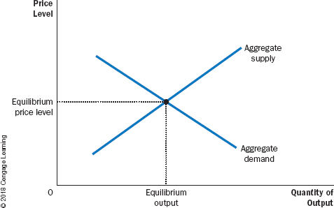
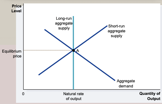
Model of Aggregate Demand and Aggregate Supply
the model that most economists use to explain short-run fluctuations in economic activity around its long-run trend
* On the vertical axis is the overall price level in the economy.
* On the horizontal axis is the overall quantity of goods and services.
* On the vertical axis is the overall price level in the economy.
* On the horizontal axis is the overall quantity of goods and services.
54
New cards
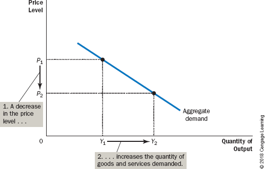
aggregate-demand curve
A curve that shows the quantity of goods and services that households, firms, and the government want to buy at each price level
* a fall in the economy’s overall level of prices tends to raise the quantity of goods and services demanded ad vice versa
* a fall in the economy’s overall level of prices tends to raise the quantity of goods and services demanded ad vice versa
55
New cards
Aggregate-Supply Curve
a curve that shows the quantity of goods and services that firms choose to produce and sell at each price level
* In the long run, the aggregate-supply curve is vertical, whereas in the short run, the aggregate-supply curve is upward sloping.
* In the long run, the aggregate-supply curve is vertical, whereas in the short run, the aggregate-supply curve is upward sloping.
56
New cards
Why does the Demand Curve Slope Downwards
* The Wealth Effect
* The Real Exchange Rate
* Interest Rate Effect
* The Real Exchange Rate
* Interest Rate Effect
57
New cards
Wealth Effect
When the price level falls, the dollars you are holding rise in value, which increases your real wealth and your ability to buy goods and services.
* A decrease in the price level makes consumers wealthier, which in turn encourages them to spend more.
* The increase in consumer spending means a larger quantity of goods and services demanded.
* and vice versa
* Ex. One dollar is always worth one dollar. Yet the real value of a dollar is not fixed. If a candy bar costs one dollar, then a dollar is worth one candy bar. If the price of a candy bar falls to 50 cents, then one dollar is worth two candy bars
58
New cards
The Interest Rate Effect
A lower price level reduces the interest rate, encourages greater spending on investment goods, and thereby increases the quantity of goods and services demanded.
* And vice versa
* And vice versa
59
New cards
The Real Exchange-Rate Effect
A fall in the Canadian price level causes the real exchange rate to depreciate, and this depreciation stimulates Canadian net exports and thereby increases the quantity of goods and services demanded.
* and vice versa
* \*GDP=C+I+G+NX
* and vice versa
* \*GDP=C+I+G+NX
60
New cards
Why the aggregate demand curve might shift
* Increases in expenditure shift the curve right
* Decreases in expenditure shift the curve left
\
* Increases in withdrawals shift left.
* Decreases in withdrawals shift right.
\
* If an injection increases or a withdrawal decreases
* At each possible price level, there is a higher level of expenditure than before
* If an injection decreases or a withdrawal increases
* At each possible price level, there is a
\
* Causes:
* Changes in Consumption
* Changes in Investment
* Changes in Government Purchases
* Changes in Net Exports
(Changes in I,X,G,C, not P)
61
New cards
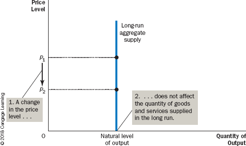
Why is the Aggregate-Supply Curve Vertical in the Long Run
* In the long run, an economy’s production of goods and services (its real GDP) depends on its supplies of labour, capital, and natural resources and on the available technology used to turn these factors of production into goods and services.
* Because the price level does not affect long-run determinants of real GDP, the long-run aggregate-supply curve is vertical,
* Because the price level does not affect long-run determinants of real GDP, the long-run aggregate-supply curve is vertical,
62
New cards
Why the aggregate supply curve might shift
* Shift to the right if there is an increase
* Shift to the left if there is a decrease
\
* Causes:
* Changes in Labour
* Changes in Capital
* Changes in Natural Resources
* Changes in Technological Knowledge
* Shift to the left if there is a decrease
\
* Causes:
* Changes in Labour
* Changes in Capital
* Changes in Natural Resources
* Changes in Technological Knowledge
63
New cards
natural level of output
The production of goods and services that an economy achieves in the long run when unemployment is at its normal rate
64
New cards
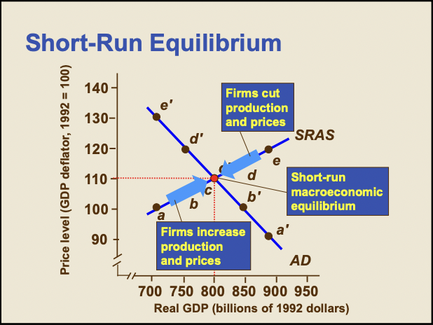
Equilibrium of agregate curves
In short-run equilibrium, Aggregate Demand (AD) = Short-Run AggregTE SUPPLY (SRAS),
* The planned expenditures of consumers, investors, etc. are consistent with the production plans of firms at the equilibrium P
* The planned expenditures of consumers, investors, etc. are consistent with the production plans of firms at the equilibrium P
65
New cards
Short Run Equilibrium
66
New cards
Long Run Equilibirum
\
67
New cards
Why does the Aggregate-Supply Curve Slope Upward in the Short Run
* The quantity of output supplied deviates from its long-run, or “natural,” level when the actual price level deviates from the price level that people expected to prevail
* When the price level rises above the expected level, output rises above its natural level, and when the price level falls below the expected level, output falls below its natural level.
* Sticky Wage Theory
* When the price level rises above the expected level, output rises above its natural level, and when the price level falls below the expected level, output falls below its natural level.
* Sticky Wage Theory
68
New cards
The Sticky-Wage Theory
According to this theory, the short-run aggregate-supply curve slopes upward because nominal wages are slow to adjust to changing economic conditions.
* In other words, wages are “sticky” in the short run.
* As price increases, it’s more profitable to produce so GDP rises
* In other words, wages are “sticky” in the short run.
* As price increases, it’s more profitable to produce so GDP rises
69
New cards
Why the SRAS Curve Might Shift
* Changes in labour, capital, natural resources, technological knowledge
* Also, price level that people expect to prevail
* When people change their expectations of the price level, the short-run aggregate supply curve shifts.
* Ex. an increase in an economy capital stock will shift the curve right
* An increases in minimum wage will shift the curve left
* Also, price level that people expect to prevail
* When people change their expectations of the price level, the short-run aggregate supply curve shifts.
* Ex. an increase in an economy capital stock will shift the curve right
* An increases in minimum wage will shift the curve left
70
New cards
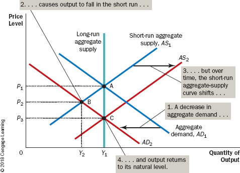
Steps for Analysing Macro Fluctuations
1. Decide whether the event shifts the aggregate-demand curve or the aggregate-supply curve (or perhaps both).
2. Decide in which direction the curve shifts.
3. Use the diagram of aggregate demand and aggregate supply to see how the shift changes output and the price level in the short run.
4. Use the diagram of aggregate demand and aggregate supply to analyze how the economy moves from its new short-run equilibrium to its long-run equilibrium.
71
New cards
Theory of Liquidity Preference
Keynes’s theory that the interest rate adjusts to bring money supply and money demand into balance
72
New cards
Money Supply Effects
* The money supply is controlled by the Bank of Canada (BoC)
* Supply of money is not affected by changes in the interest rate
\
* Curve shifts right is there is an increase in the money supply
* When supply shifts, so does demand because the shift in supply changes interest rates. Interest rate affects demand.
* Supply of money is not affected by changes in the interest rate
\
* Curve shifts right is there is an increase in the money supply
* When supply shifts, so does demand because the shift in supply changes interest rates. Interest rate affects demand.
73
New cards
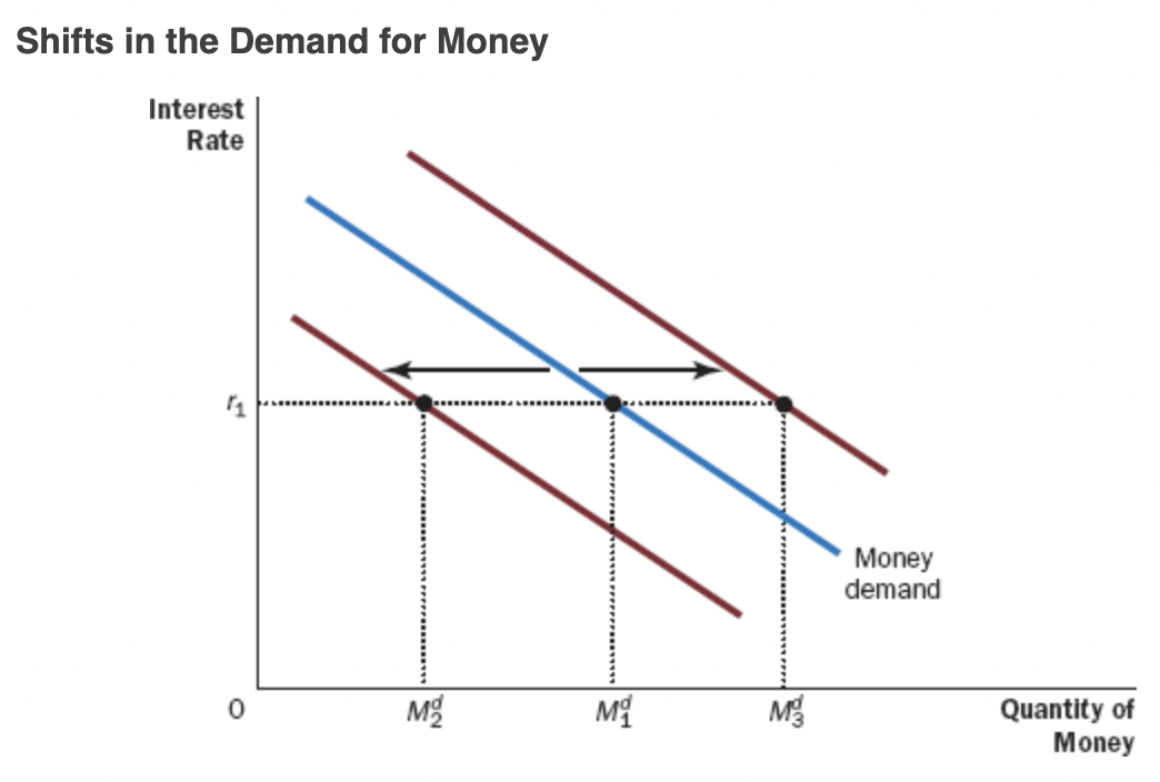
Money Demand Effects
* The liquidity of money explains the demand for it: People choose to hold money instead of other assets that offer higher rates of return because money can be used to buy goods and services.
* Demand depends on interest rate
* the interest rate is the opportunity cost of holding money.
* An increase in the interest rate raises the cost of holding money and, as a result, reduces the quantity of money demanded.
* A decrease in the interest rate reduces the cost of holding money and raises the quantity demanded
\
* Shifts right if P of real GDP increase
* Shifts left if P or real GDP decreases
74
New cards
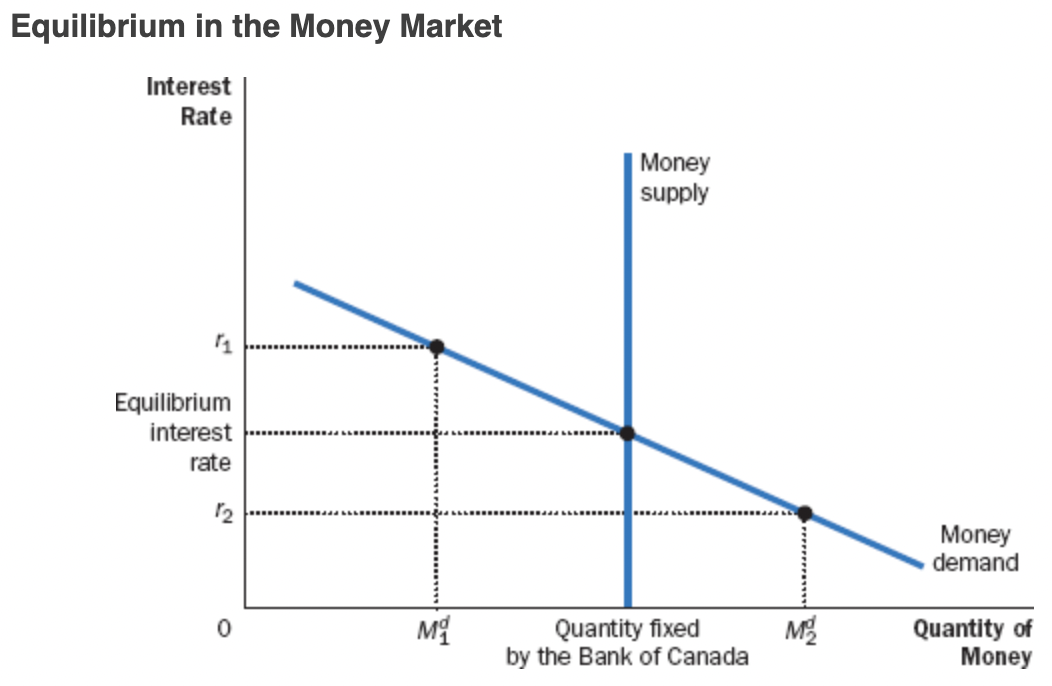
Equilibrium in the Money Market
* According to the theory of liquidity preference, the interest rate adjusts to balance the supply and demand for money.
* If the interest rate is higher (r1), there is an excess supply of money,
* Downward pressure on interest rates, causing the quantity demanded of money to rise, moving it back toward equilibrium quantity supplied
* If the interest rate is lower (r2), there is excess demand for money,
* upward pressure on interest rates, causing the quantity demanded of money to fall, moving it back toward equilibrium quantity supplied
\
Interest Rate Effect:
* A higher price level raises money demand.
* Higher money demand leads to a higher interest rate.
* A higher interest rate reduces the quantity of goods and services demanded.
75
New cards
Shift in Supply Graph
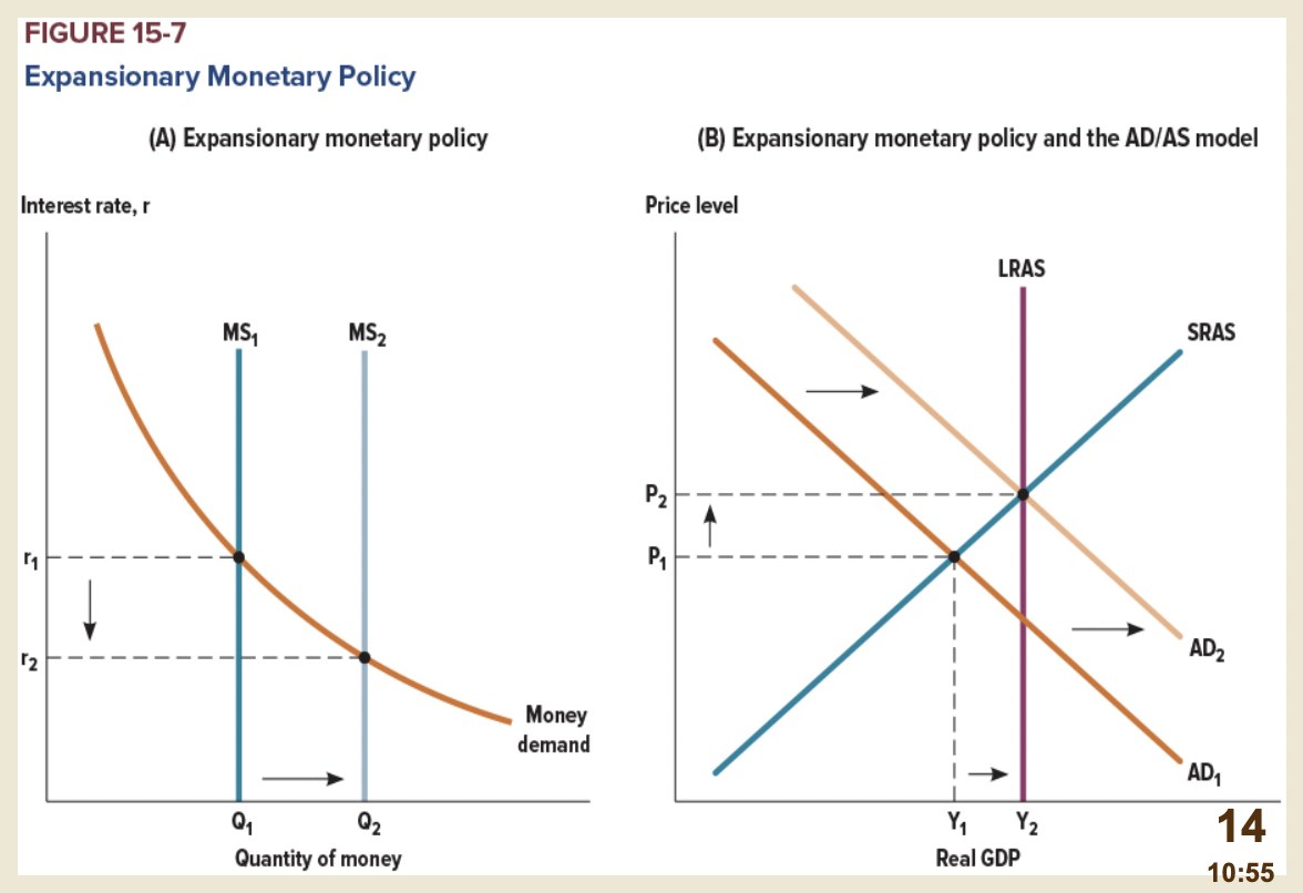
* *When the Bank of Canada increases the money supply, it lowers the interest rate and increases the quantity of goods and services demanded for any given price level, shifting the aggregate-demand curve to the right.*
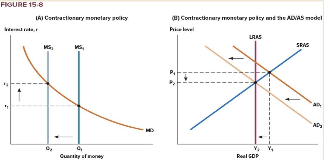
* *Conversely, when the Bank of Canada contracts the money supply, it raises the interest rate and reduces the quantity of goods and services demanded for any given price level, shifting the aggregate-demand curve to the left*.
* *Conversely, when the Bank of Canada contracts the money supply, it raises the interest rate and reduces the quantity of goods and services demanded for any given price level, shifting the aggregate-demand curve to the left*.
76
New cards
Flexible Exchange Rate
A policy by which the value of the exchange rate is allowed to vary without interference by the central bank
77
New cards
Expansionary monetary policy
* Works by reducing interest rates and stimulating investment spending
* The economy in a recessionary or a negative output gap
* The economy in a recessionary or a negative output gap
78
New cards
Contractionary Policy
* Monetary measure to reduce government spending or the rate of monetary expansion by a central bank.
* Restrictive monetary policy
* Restrictive monetary policy
79
New cards
Stabilisation Policy
Deliberate, conscious effort of the government to intervene in the macroeconomy with an eye toward influencing the course of Equilibrium P or Q (real GDP)
80
New cards
Fiscal policy
The setting of the level of government spending and taxation by government policymakers
81
New cards
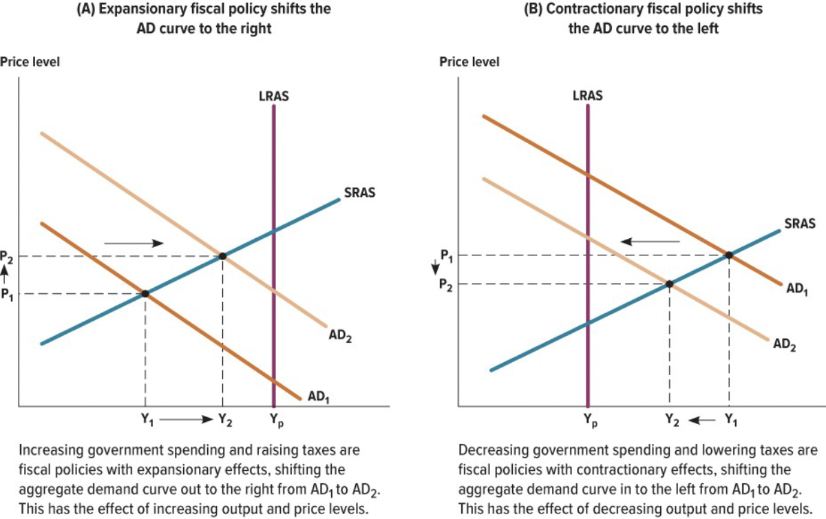
Expansionary and Contractionary Fiscal Policy Shifts
* Expansionary shitfs the AD curve right
* Contractionary shifts the AD curve left
* Contractionary shifts the AD curve left
82
New cards
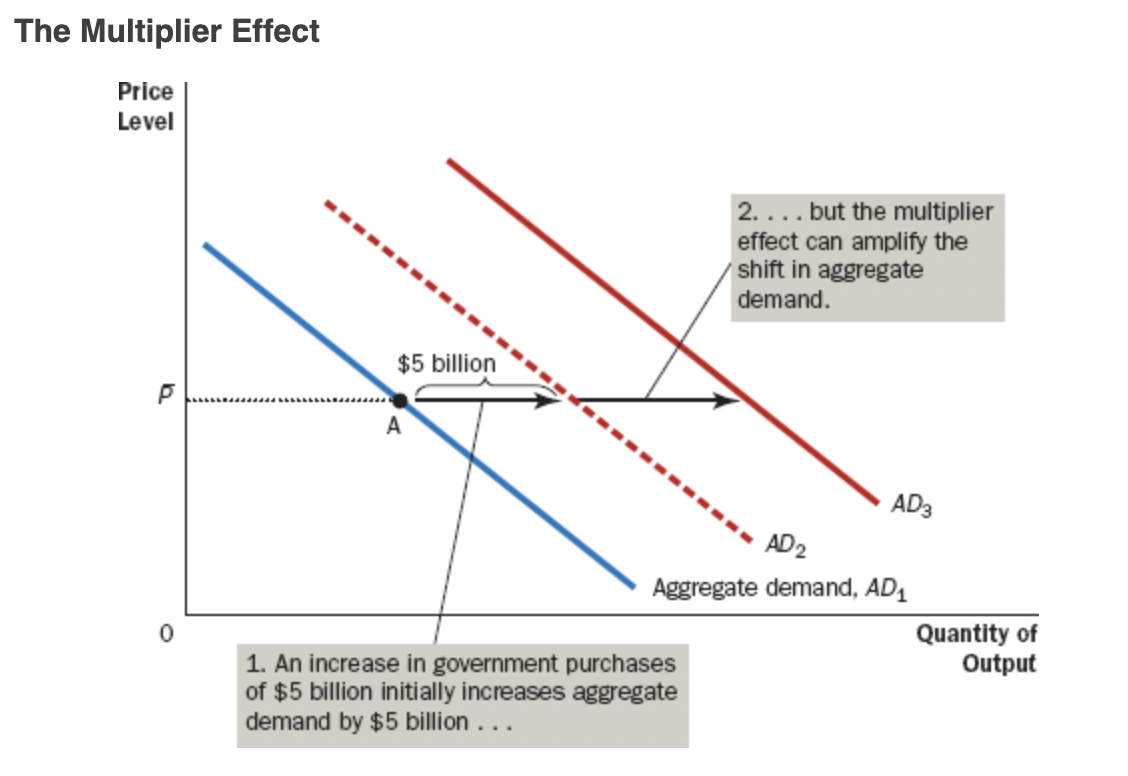
Multiplier Effect
The additional shifts in aggregate demand that result when expansionary fiscal policy increases income and thereby increases consumer spending
* The basic idea is that if the government increases spending (which it is doing now big time), this increase in spending has an effect on AD that causes it to expand again and again
* Ultimately by much more than the initial expansion of AD
* Geometrically, it is the magnitude of the horizontal shift in AD
\
* When consumer spending rises, the firms that produce these consumer goods hire more people and experience higher profits.
* Higher earnings and profits stimulate consumer spending once again, and so on.
* Thus, there is positive feedback as higher demand leads to higher income, which in turn leads to even higher demand
\
* Interpretation: the change in total spending (C + I + G + NX) which results from a $1 change in government spending.
* The higher (lower) the multiplier, the greater (lesser) the response
\
83
New cards
Formula for the Spending Multiplier
* Value of multiplier = Δ aggregate expenditure /Δ G
* MPC: marginal propensity to consume
* The fraction of extra income that a household consumes rather than saves
* Ex. For example, suppose that the marginal propensity to consume is
3/4. This means that for every extra dollar that a household earns, the household spends $0.75 (3/4 of the dollar) and saves $0.25
* With an *MPC* of 3/4, when the workers and owners of the construction firms earn $5 billion from the government contract, they increase their consumer spending by 3/4×$5billion, or $3.75 billion.
* This goes on. Becomes MPC×(MPC×$5billion). These feedback effects go on and on.
* Multiplier = (1 + MPC + MPC 2+ MPC3 + …) x 5 billion
* Multiplier= 1/(1-MPC)
* The government-spending multiplier tells us the demand for *Canadian-produced* goods and services generated by each additional dollar of government expenditure.
* *marginal propensity to import (MPI)*
* The relevant formula for the government-purchases multiplier in an open economy is:
* Multiplier= 1/(1-MPC+MPI)
84
New cards
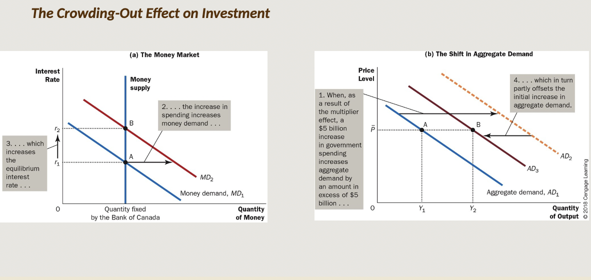
The Crowding-Out Effect on Investment
The offset in aggregate demand that results when expansionary fiscal policy raises the interest rate and thereby reduces investment spending
* In the OUTPUT market, the increase in G, amplified by the multiplier effect, results in a new equilibrium with an increase in both P and real GDP
* In the MONEY market, these changes cause an expansion in the demand for money, resulting in an increase in the equilibrium interest rate
* Back in the OUTPUT market, this increase in the interest rate causes a decrease in I spending, which causes a leftward shift in the AD curve
* This is the ‘crowding out’ part
* Net effect: the impact of the fiscal stimulus is partially OFFSET but probably not by 100 %
\
When the government increases its purchases by $5 billion, the aggregate demand for goods and services could rise by more or less than $5 billion, depending on whether the multiplier effect or the crowding-out effect on investment is larger. The crowding-out effect pushes the aggregate-demand curve in the opposite direction and, if large enough, could result in an aggregate-demand shift of less than $5 billion
85
New cards
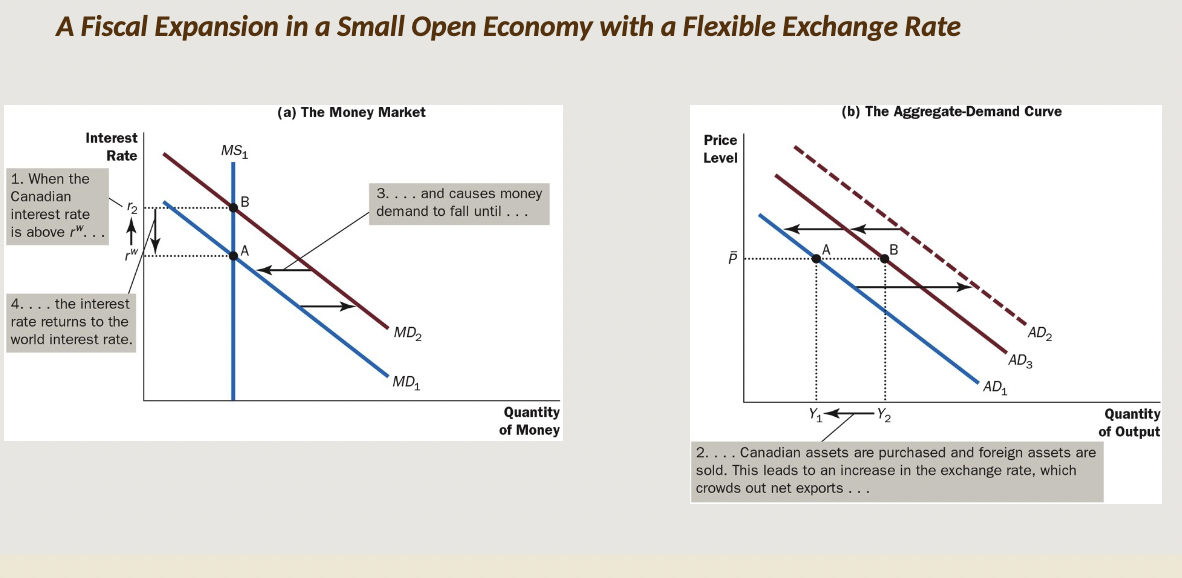
Crowding Out Effect Open Economy
* In the OUTPUT market, the increase in G, amplified by the multiplier effect, results in a new equilibrium with an increase in both P and real GDP
* In the MONEY market, these changes cause an expansion in the demand for money, resulting in an increase in the equilibrium interest rate
* Back in the OUTPUT market, this appreciation in the Canadian $ causes a decrease in NX spending, which causes a leftward shift in the AD curve
* This is the ‘crowding out’ part
* Net effect: this instance of crowding out can amplify the other case (involving I spending), and further OFFSET the fiscal stimulus
\
*In a small open economy, an expansionary fiscal policy causes the dollar to appreciate. Because this appreciation of the dollar causes net exports to fall, there is an additional crowding-out effect that reduces the demand for Canadian-produced goods and services. In the end, fiscal policy has no lasting effect on aggregate demand*.
86
New cards
crowding-out effect on net exports
The offset in aggregate demand that results when expansionary fiscal policy in a small open economy with a flexible exchange rate raises the real exchange rate and thereby reduces net exports
87
New cards
Automatic Stabilizer
Fiscal policy that is built into the government’s tax and expenditure apparatus that self-activates
Changes in fiscal policy that stimulate aggregate demand when the economy goes into a recession, without policymakers having to take any deliberate action
\
* Tax system, Government Spending:
* When in a recession, UI payments increase and total tax revenue decreases
* AD shifts rights. But not sufficient to bring about an end to the recession
* When beyond potential GDP, UI payments decrease and total tax revenue increases
* AD shifts left.
88
New cards
Deficits and debt
* Fiscal Deficit = T – G < 0
* Fiscal Surplus = T – G > 0
\
* Both quantities typically expressed as a share of GDP, as GDP (= aggregate income) is the means to repay it.
* Deficits are financed by issuing government bonds
* Fiscal Surplus = T – G > 0
\
* Both quantities typically expressed as a share of GDP, as GDP (= aggregate income) is the means to repay it.
* Deficits are financed by issuing government bonds
89
New cards
Debt vs Deficit Definitions
* Debt is a STOCK quantity referring to total amount owed
* No time frame
* Sum of all prior deficits and surpluses
* Deficit is a FLOW quantity referring to shortfall PER TIME PERIOD
* No time frame
* Sum of all prior deficits and surpluses
* Deficit is a FLOW quantity referring to shortfall PER TIME PERIOD
90
New cards
Benefits of debt-financed deficits
VERY politically popular because it’s “free extra spending”
* Actually, it is not
* Address negative AD and/or SRAS shocks
* Can finance investments in infrastructure that increase AS in both the short-run and the long-run
* If it’s PRODUCTIVE public investment
* Actually, it is not
* Address negative AD and/or SRAS shocks
* Can finance investments in infrastructure that increase AS in both the short-run and the long-run
* If it’s PRODUCTIVE public investment
91
New cards
Costs of debt-financing
* Payment of interest
* Re-payment of principal
* Future generations only are affected
* Crowding-out of private investment spending
* Re-payment of principal
* Future generations only are affected
* Crowding-out of private investment spending