Lecture 11 : GL An introduction to Time series forecasting

time series

= sequence of data points observed at successive, equally spaced points in time (fixed periodicicty : hourly, daily, monthly)

scalar on function regression

input : function / time series

output : numerical

is a type of statistical model used when you want to predict a single number (a scalar) using a predictor that is a curve or a shape (a function).

eg : time series of height prokected of a child, you map the data on an annual basis, and you want to predict the height at a certain age

time series classification

• input : function/ time series

• output : categorical

→ feature based : These methods transform the raw time series into a set of summary statistics or features. Once the time series is represented as a vector of numbers, any standard machine learning classifier (like Random Forest or XGBoost) can be used.

→ distance beased : These methods rely on a similarity measure (a distance function) to compare two raw time series. Instead of looking for specific properties like "slope" or "mean," they compare the actual shapes of the sequences.

categorical time series analysis

input : past values of same and or other time series

output : categorical element of time series

catgeorical in nature

binarizing continuous targets

time series components :

• periodic patterns and autocorrelation

generalized linear models : multinomial/logistic regression

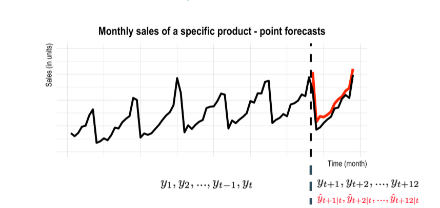
time series regression / forecasting

input : past values of same and or other time series

output : numerical lemeents of time series

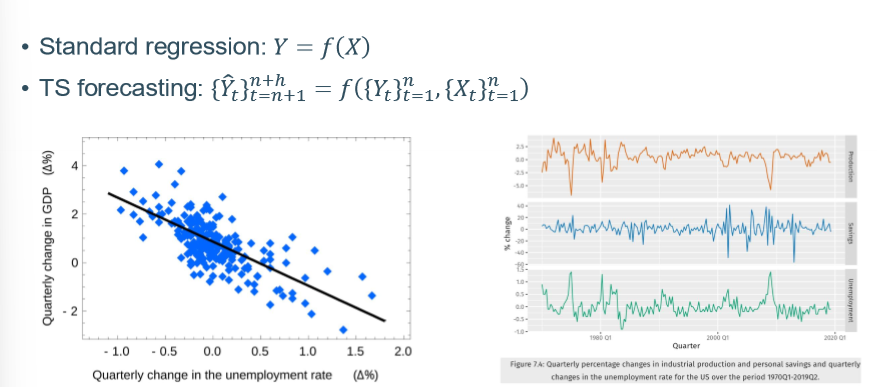
standard regression vs time series forecasting

standard regression Y = f(x) → time is not taken into account, it assumes that all observations are independent

TS forecasting : Predicts future values of a variable based on its own past values. It assumes observations are dependent on what happened before

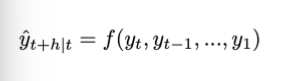
classical time series forecasting methods : univariate

= only used historical values of the time series itself to make forecasts

→ additive : yt = St + Tt + Rt

→ multiplicative : yt = St*Tt* Rt → equivalent to log(yt) = log(St) + log(Tt) + log (Rt)

(multiplicatibe : when variability is dependent on the level of the time series)

autocorrelation

measures the linear relationship between lagged values of a time series

ACF plots

autocorrelation function

TS forecasting : historical events : 1982 the first M(akridakis) competition

• first true forecasting competition : multiple people could submet entries

• 1001 time series

TS forecasting : historical events : 1982 the first M(akridakis) competition : main findings

• simple forecasting methods often produce more accurate forecasts than complex methods → shoft in focus from in-sample model fit to out-of sample forecasting performance (on unseen data)

• cobining forecasts typically results in improved forecast accuracy : combine vs identify and fit single model that describes the data generating proces

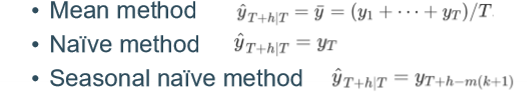
univariate time series forecasting techniques : simple forecasting methods

mean method

naïve method : taking the last observed value as proxy

seasonal naïve method :

TS forecasting : historical events : 1998 the M3 competition

• aim = updating frist M competition taking into account new methods

• 303 time series

focus of forecasting community → fine-tuning combination schemes and automated forecasting methods

TS forecasting : historical events : 1998 the M3 competition : main findings

• opinions differ regarding evidence as to whether simple methods outperform complex ones

• additional evidence of the benefit of combining multiple forecasts = ensembling

univariate time series forecasting technques : exponential smoothing

forecasts = weighted average of past observations, with the weights decaying exponentially as the observations get older

description of trend and seasonalily + how they enter the smoothing methode (in additive or multiplicative manner)

which exponential smoothing formulation to use

• ad hoc → detailed inspection of time series

• ETS :

• → state space model formation → statistical framework that underlies exponential smoothing methods

• → automatic model selection algorithm (based on minimizing AIC )→ ets()

ETS

state spare model formulation → statistical framework that underlies exponential smoothing methods

automatic model selection algorithm (based on minimizing AIC) → ets()

univariate time series forecasting technques : exponential smoothing : different exponential smoothing methods

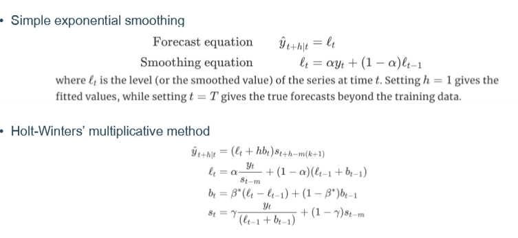
• simple exponential smoothing

• holt winter’s multiplicative method

univariate time series forecasting technques :ARIMA

describes (seasonal) autocorrelations in the data

automatic model selection algorithm (based on minimizing AIC)

→ auto.arima()

which other univariate time series forecasting techniques exist ?

• hierarchical time series forecasting

• nnetar (neural entwork time series forecasts)

neural networks in M3 and NN3

only one NN submission in M3 → it did relatively poorly

NN3 ; Sven Crone organized a subsequent NN competition in 2006

• 111 of the monthly M3 series

• over 60 algorithms were submitted, none outperformed original M3 contestants

consensus in forecasting community

• NN and other data hungy ML methods are not well suited to univariate time series forecasting

evolutions in time series forecasting

combining simple forecasting methods

• fine-tuning combination schemes and automated forecasting methods

big data era

• demand sensing + machine learning (ML) methods

from local to gloal time series forecasting models

• keeping up with the advances in ML → deep learning

from point to probabilistic forecasting

• quantify forecast uncertainty

big data era = demand sensing (and other time series problems where external variables are available)

not only use prior demand data but alse use ‘a wide range of demand signals that reflect changing customer preferences as they unforl”

examples of demand sensing signals

• promotional data

• weather predictions

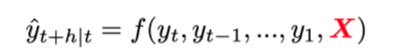
big data era : using external variablkes (xreg)

TSX (extend classical time forecasting, combining it with a xreg)

• different flavors of auto.anima() or ets() + lm(residual-xreg)

• useful if limited number of xreg, eg promotion dummy variablke

• if xreg contains many variables (potentially due to unknown lag order)

• → need for variable selection eg hybrid stepwise aproach

• → we end up with p » n scenario rather quickly → limited hustorical data in proportion to potential leading indicators + unknown lag ordder

ML (bc you need to look further than the standard methods)

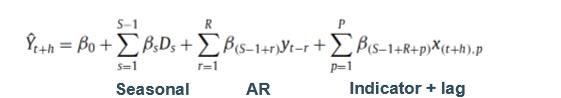
• add TS fetaures to xreg (AR terms, trend, seasonal dummies)

big data example : problem discription and objective

tactical forecasting in supply chain management

• supports planning for inventory, scheduling production, and raw material purchase,

• forecasts up to 12 months ahead dor 4 different time series

• large set of potentially relevant macro economic indicators

objective : improve tactical sales forecasting by using macro-economic leading indicators to replace judgemental (human) adjustments to incorporate macro-economic info

solution : LASSO to automatically select both the tupe of leading indicators, as well as the order of the lead dor each of the selected indicators + unconditional forecasting setup

M4 competition

forecast accuracy

forecast uncertainty → 95% PI

dataset was way larger (than M3)

from local to global time series forecasting models : local

= train one model for each time series

• estimate model parameters independentely for each time series

• limited availability of training data → only models with small number of free parameters can be estimated reliably

• well known local methods : ETS and ARIMA

from local to global time series forecasting models : Global

= train one model jointly across time series

• estimate model parameters jointly from all available time series

• large training data set → DL model with mollions of parameters can be used

from local to global time series forecasting models : ML methods such as ANN and tree-based ensembles can be used both in global and local settings

local + ML : mixed results (univariate vs xreg)

global + ML : good results in M4 and M5 competitions

distinction local VS global is complementary to distinction between univariate vs multivariate

→ global metods do not imply a particular (in-)dependence structure between the time series vs explicitly modeled dependency structure between time series in multivariate methods

from point to probalistic forecasting : why quantify uncertainty

• no need for forecasting in a world without uncertainty

• forecast uncertainty frequently crucial to optimal decision making (eg safety stocks)

which are the sources of uncertainty in forecasting using time series models

• random error term

• parameter estimates

• choice of model for the historical data

• continuation of the historical data generating process into the future

which sources of uncertainty to model driven prediction intervals for time series such as ETS account for

only for random error term

M4 competition results

conclusion = hybrid is the way forewarde (vb pure ML)

local model-driven component - A model is only as good as its assumptions

• model a limited set of patterns defined by the assumptions (eg trend or no trend)

• parsimoniously parametrized and therefore nedd little data to be accurately fitted

global data-driven component - a model is only as good as the data it is fed

• no strong structural assumptions

• flexible (large number of parameters) at the cost of being data hungry

N-beats

doubly residual stacking -backcast, partial forecasts

sequential analysis of raw input time series

very deep network

when not to go global

strategic forecasting problem

• high level aggregated

• decision problems : long term capacity planning (investments), market entry

• fit in domein knowledge

when to go global

decision problems : inventory management, capacity scheduling

enough data is available to learn complex patterns

too many time series and edge cases to design specific methods → ratio of forecasters/ time series « 1

why is deep learning architectures for time series forecasting an active field of research

flexibility

incorporating domein-specific ingedients such as forecast stability

• customize loss functions

• N-BEAT-S

direct probabilistic forecasting

• parameters of probability distribution as outputs → loss = negative log-likelihood

• N-N-BEATS

N-BEATS -S forecast updating and instability → cost and benefits

forecast updating

benefits : more accurate period-specific forecasts due to shorter forecast horizon

costs : induces instability which lead to revisions to supply plans

N-BEATS -S =

N-BEATS +

adding forecast instability component to loss functin to optimize forecasts from both

• traditional forecast accuracy

• forecast stability perspective

enter the M5 competition

= the first open data set that can be considered representative for real-world operational forecasting problems (meta-data, covariates, hierarchical structure, intermittency)

separate accuracy and uncertainty tracks

LightGBM and XGBoost in M5

hugely popular in M5

• missing value treatment

• speed

• good default and trobust performance

• easy to integrate covariates

M5 contestants did'n’t modify the core algorithms

characteristics of M5 winning method

22 Global LightGBM mmodel per store

equally weighted ensemble of recursive and non-recursive models

different models have dufferent yperparameters and input features

many decisions are based on expertise and feature selection procedures

→ heavy ensembling of tree-based learners

the future of time series forecasting

efficiency and stability of training and prediction

• N-BEATS state of the art performance on M3 and M4 competition data sets

• → no time series specific eleents

• → ensembling (180 different N-BEATS networks)

• model innovation vs brute force ensembling = adding more compute power

• hybrid architectures

• → time series specific elements + global modeling approach

• → leveraging robustness and stability of local classical tie series methods

the future of time-series forecasting - pre-trained global deep learning models = transfer learning

train on source data set(s), deploy on new target data set(s) (after fine-tuning)

pre-trained models on heterogeneous datasets (eg pooled over multiple customers of software vendor)

use data-driven DL forecasting models even if only limited training data is available (few shot transfer learning)

future of time-series forecasting : zero short transfer learning

application of N-BEATS in zero shot learning setting

• train on source data set

• deploy on new target data set

• no fine-tuning