Signals, Spectra, Signal Processing

Voice frequency

300 Hz - 3kHz

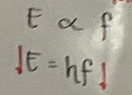
Equation relating energy and frequency

Planck’s Equation

Fidelity

Ability of a system to create an exact replica of the input at the output

Parts of a Communication System

Source:

• Transducer

• Transmitter

Channel

Destination

• Receiver

• Transducer

Transducer

• Device that changes one form of energy to another

• Trans: “to change”

• Ducer: “induce”

Transmitter

Collection of circuits that prepares the signal for transmission

Channel

• This is where noise is added

• Types:

  • Guided - Waveguides (for high frequqncies), Transmission Lines

  • Unguided - Free space (Antenna - radiator)

Receiver

Collection of circuits that extracts the message from the signal

Hearing frequencoes

20 Hz - 20kHz

Guglielmo Marconi

1st person to achieve transatlantic radio transmission

wireless

Radio means

to share

Communicare means

Information

Meaning to be sent

Data

Representation of the information

Signals

• Message

• Carrier of information

• Physical quantity or variable, and typically, it contains information about the behavior or nature of the phenomenon

Visible light frequency and wavelength

THz, μm

Microwave wavelength

millimeters

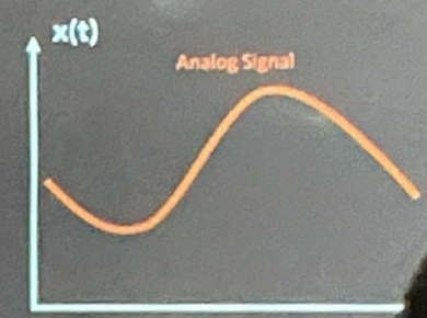
ANALOG SIGNALS

• Continuous in both time and amplitude

• Electrical properties used are voltage, followed closely by frequency, current and charge.

DIGITAL SIGNAL

• Discrete in both time and amplitude

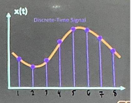
Sampling

• Selecting values of an analog signal at discrete time instants.

discrete-time

All digital signals are

Quantization

Averaging the amplitude of discrete time signal to make it discrete time-amplitude

Coding

Assigning codes to represent the levels of the signal

Analog-to-Digital Conversion

1. Sampling

2. Quantization

3. Coding

Advantage of Digital Signal

• Digital data will be much easier to store than continuous data.

• Easier to process because the data are finite.

• For security! Data can be encrypted and decrypted.

• Cross-talk and the probability of error is a rare occurrence.

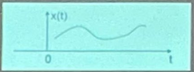
Continuous-Time

• Represented by x(t)

• Continuous and real in domain and range

Discrete Time

• Represented by x[n]

• Often identified as a sequency of numbers

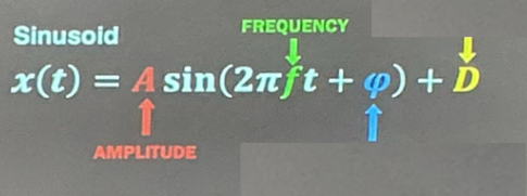
Equation of a continuous time signal

x(t) = Asinθ

θ, Angular Displacement

• Is the phase

• equal to ωt (angular velocity times time)

ω, Angular frequency/velocity

• in rad/sec

• equal to 2πf

f, frequency

• also called the Cyclic Frequency

• in cycles/sec

Phase Shift / Horizontal Shift

(the blue indicator) shows

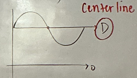
Vertical Shift

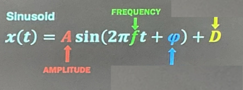
(the yellow indicator) shows

T, period

• Reciprocal of frequency, 1/f

• equal to 2π/ω

• in sec/cycle

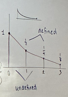
Explicit notation for the nth value of the sequence

• Set-builder notation

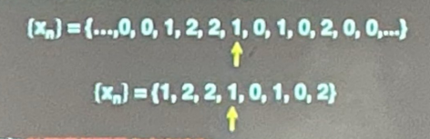
Listing the nth value of the sequence

• Roster Method

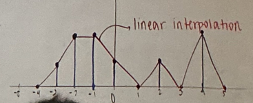
• Interpolation: Estimating an unknown value that lies between two known values.

Aliasing

• It refers to the effect produced when a signal is imperfectly reconstructed from the sampled signal.

• It occurs when a signal is not sampled at a high enough frequency to create an accurate representation.

• Too few samples

• Undersampling

Anti-aliasing

• Too many samples

• Oversampling

• Causes fold over distortion

Crossover distortion*

• introduces unwanted frequency components into the transmitted signal, which can degrade the quality of the received signal.

• occur when a signal passes through a nonlinear device, such as an amplifier, particularly when the signal transitions through the zero-voltage region.

SAMPLING THEOREM

"A bandlimited continuous-time signal can be sampled and perfectly reconstructed from its samples if the waveform is sampled over twice as fast as its highest frequency component."

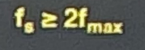
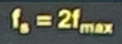
Nyquist Frequency, fs

• Maximum frequency that can be sampled by a sampling frequency

Nyquist Rate

Minimum frequency that can sample a signal with minimal aliasing

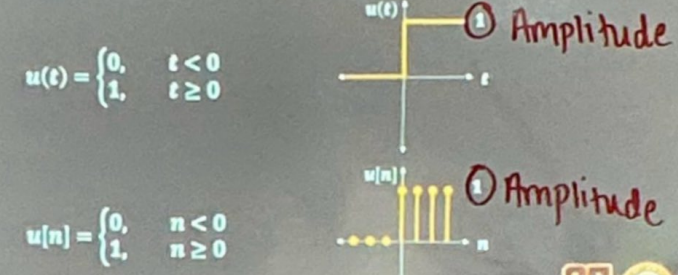
Unit Step

Singularity function also called as the Heaviside Step Function

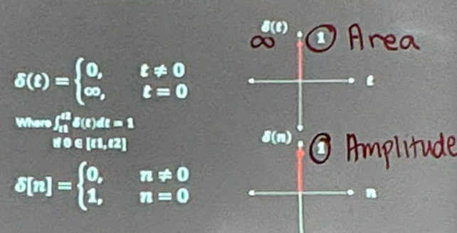
Unit Impulse Function

Singularity function also called as the Dirac’s Delta Function

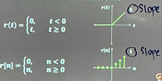
Unit Ramp Function

Singularity function also called as the Rectified Linear Unit

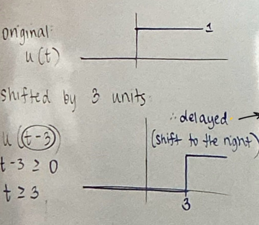
Delayed Time Shifting

• Default if not specified as “left or right time shifted”

• shift = subtraction

• Shift to the right

• t → t - a

Advanced Time Shifting

• Shift to the left

• t → t + a

Time Reversal

• Flip / mirror with respect to t = 0

• Reflecting about the y-axis

• t → -t

Expansion Time Scaling

• Oversampling

• t → t/k

• n → n/k

Compression Time Scaling

• Undersampling

• t → kt

• n → nk

work on every choice first then compare to the given if they match

For signal manipulation problems:

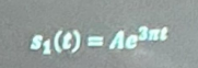
Real signal

Signal is purely real

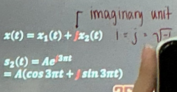
Complex Signal

Signal has an imaginary part

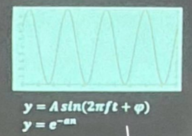
Deterministic Signal

• Signals whose values are completely specified for any given time.

• Can be expressed mathematically

• Exhibits no uncertainty

• Includes all even and odd signals

Random Signal

• Signals that take random values at any given time.

• Non-deterministic

• Stochastic

• Cannot be expressed mathematically

• Uses probability

• Exhibits uncertainty

• Includes white noise

Even Signal

• Symmetrical about the y-axis

• if x(-t) = x (t)

• if x[-n] = x[n]

• 1 fold function

Odd Signal

• Symmetrical about the origin

• if x(-t) = -x(t)

• if x[-n] = -x[n]

• 2 fold function

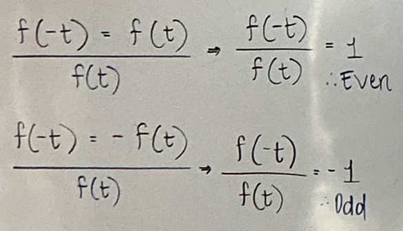
Technique for even and odd function

Periodic Signal

• Repeating

• x (t + T) = x(t); T(period) can be irrational

• x [n + N] = x[n]; N cannot be irrational

Aperiodic Signal

• Non-repeating

Which statement is always true

Fundamental Period

• The LCM of the periods of the components
  ex. LCM (60°, 90°) = 180° = π

• the smallest positive time interval after which the entire function repeats exactly.

To know if the function with different components are periodic or aperiodic:

• Solve the T period of each component

• Identify if each period is irrational or rational

• If both are irrational or both rational: periodic

• If they differ (1 rational, 1 irrational): aperiodic

Energy Signal

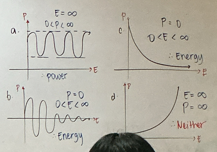
• Finite energy (duration): 0 < E < ∞

• Finite amplitude

• Power = 0 as t → ∞

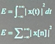
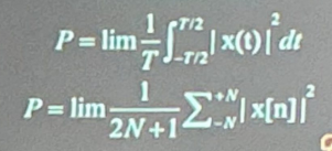
Power Signal

• Not limited in time

• Non-zero for infinite amount of time

• Finite power (amplitude): 0 < P < ∞

• E = ∞ as t → 0

Examples of Power and Energy functions

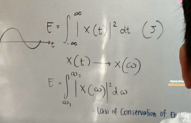
Parseval’s Theorem

• Total energy of a signal is the same whether you calculate it in the time domain or in the frequency domain

• Energy in time domain = Energy in frequency domain

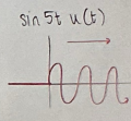
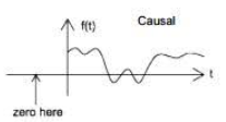
Causal Signal

• Signal that does not start before t = 0

• cause → effect

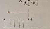
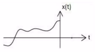
Anti-causal Signal

• Signal that ends at t = 0

• effect → cause

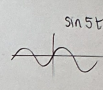
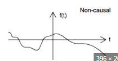
Non-causal

• Starts before t=0 and continues after t=0

• does not follow the Law of Cause and Effect