MCAT Physics and Math - Data-Based and Statistical Reasoning

691

Measures of central tendency

describe the middle(s) of a sample

mean / (arithmetic) average

calculated by adding up all of the individual values within the data set and dividing the result by the number of values

where x_i to x_n are the values of all of the data points in the set and n is the number of data points in the set

good indicator of central tendency when all of the values tend to be fairly close to one another

outlier

extremely large or extremely small value compared to the other data values

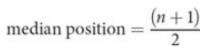
median

midpoint, where half of data points are greater than the value and half are smaller; data set must first be listed in increasing fashion

where n is the number of data values

least susceptible to outliers, but may not be useful for data sets with very large ranges or multiple modes

mode

the number that appears the most often in a set of data; may be multiple, one or none; represented graphically as peaks; not directly used as measure of central tendency but relationships can be enlightening

normal distribution / bell curve

mean = median = mode

68% of the distribution is within one standard deviation of the mean, 95% within two, and 99% within three

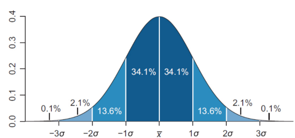
standard distribution

mean of zero and a standard deviation of one, can be extrapolated from any normal distribution

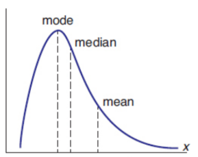
skewed distribution

one that contains a tail on one side or the other of the data set; visual shift in the data appear opposite the direction of the skew

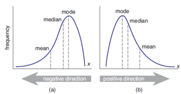
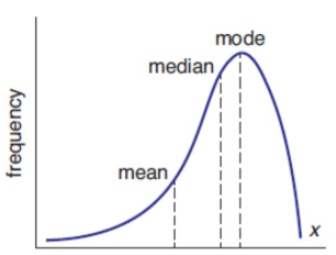
negative skew

tail to left

mean < median < mode

positive skew

tail to right

mode < median < mean

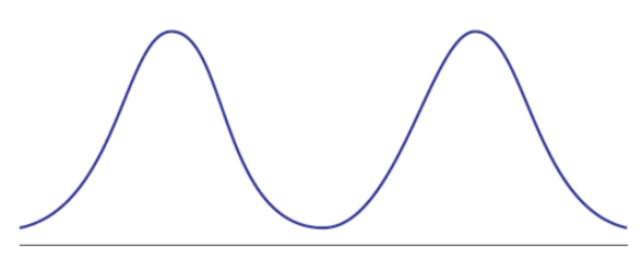
bimodal

distribution containing two peaks with a valley in between; might have only one mode if one peak is slightly higher than the other; can often be analyzed as two separate distribution

range

difference between its largest and smallest values; does not consider the number of items of the data set, nor the placement of any measures of central tendency; possible to approximate the standard deviation as one-fourth

range = x_max − x_min

Quartiles

divide data (when placed in ascending order) into groups that comprise one-fourth of the entire set

Calculate quartiles

To calculate the position of the first quartile (Q1) in a set of data sorted in ascending order, multiply n by ¼.

median (Q2)

To calculate the position of the third quartile (Q3), multiply the value of n by ¾.

• If this is a whole number, the quartile is the mean of the value at this position and the next highest position.

• If this is a decimal, round up to the next whole number, and take that as the quartile position.

Interquartile range

calculated by subtracting the value of the first quartile from the value of the third quartile

IQR = Q₃ – Q₁

outlier

Any value that falls more than 1.5 interquartile ranges below the first quartile or above the third quartile OR that lies more than three standard deviations from the mean

may be: true statistical anomaly, measurement error, distribution that is not approximated by the normal distribution

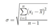
Standard deviation

calculated by taking the difference between each data point and the mean, squaring this value, dividing the sum of all of these squared values by the number of points in the data set minus one, and then taking the square root of the result

where σ is the standard deviation, xi to xn are the values of all of the data points in the set, is the mean, and n is the number of data points in the set.

independent events

have no effect on one another

Dependent events

have an impact on one another, such that the order changes the probability

Mutually exclusive outcomes

cannot occur at the same time

exhaustive

there are no other possible outcomes

probability of two or more independent events

product of their probabilities alone

P(A ∩ B) = P(A and B) = P(A) × P(B)

probability of at least one of two independent events

equal to the sum of their initial probabilities, minus the probability that they will both occur.

P(A ∪ B) = P(A or B) = P(A) + P(B) − P(A and B)

Hypothesis testing

begins with an idea about what may be different between two populations

null hypothesis

always a hypothesis of equivalence; says that two populations are equal, or that a single population can be described by a parameter equal to a given value

alternative hypothesis

a hypothesis contrary to the null hypothesis

nondirectional

alternative hypothesis that the populations are not equal

directional

alternative hypothesis that the mean of population A is greater than the mean of population B

z- or t-tests

most common hypothesis tests which rely on the standard distribution or the closely related t-distribution

test statistic

calculated and compared to a table to determine the likelihood that that statistic was obtained by random chance

p-value

the likelihood that that statistic was obtained by random chance under the assumption that our null hypothesis is true

significance level (α)

comparison of p-value; 0.05 is commonly used

p-value > α, fail to reject the null hypothesis - not a statistically significant difference between the two populations

p-value < α, reject the null hypothesis - there is a statistically significant difference between the two groups

type I error

the likelihood that we report a difference between two populations when one does not actually exist; probability is α; false positive

type II error

incorrectly fail to reject the null hypothesis; probability is β; false negative

power

The probability of correctly rejecting a false null hypothesis; equal to 1 − β

confidence

probability of correctly failing to reject a true null hypothesis

Results of Hypothesis Testing

Confidence intervals

essentially the reverse of hypothesis testing; determine a range of values from the sample mean and standard deviation

Charts

present information in a visual format and are frequently used for categorical data

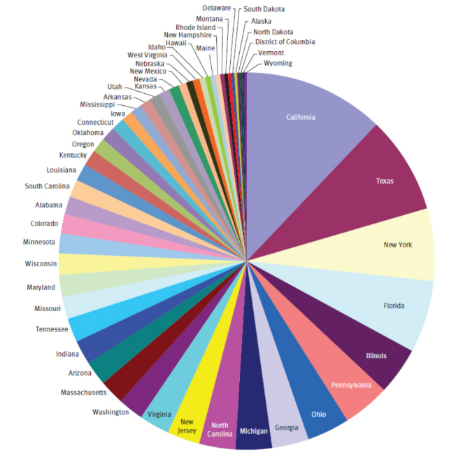
Pie / circle charts

used to represent relative amounts of entities and are especially popular in demographics; may be labeled with raw numerical values or with percent values

as the number of represented categories increases, the visual representation loses impact and becomes confusing

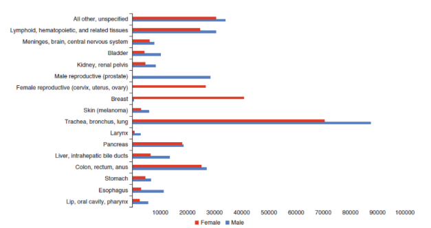
Bar charts

used for categorical data, which sort data points based on predetermined categories; may then be sorted by increasing or decreasing bar length; length of a bar is generally proportional to the value it represents

breaks should be avoided in the chart because of the potential to distort scale

Histograms

present numerical data rather than discrete categories; particularly useful for determining the mode of a data set because they are used to display the distribution of a data set

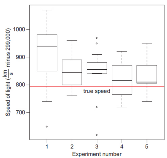
Box plots

used to show the range, median, quartiles and outliers for a set of data

box-and-whisker

a labeled box plot; box is bounded by Q1 and Q3; Q2 is the line in the middle of the box; ends of the whiskers correspond to maximum and minimum values of the data set

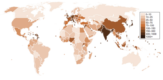
Maps

data can be illustrated geographically; relatively easy to comprehend and may show geographic clustering for some data

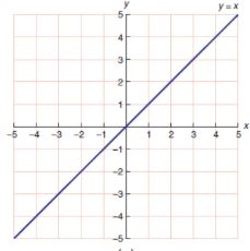
Linear graphs

show the relationships between two variables; curve may be linear, parabolic, exponential, or logarithmic; axes of a linear graph will be consistent in the sense that each unit will occupy the same amount of space

linear shape graph

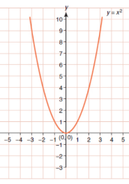
Parabolic graph

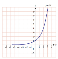
Exponential graph

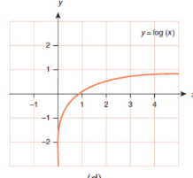
Logarithmic graph

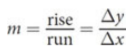
Slope (m)

change in the y-direction divided by the change in the x-direction for any two points

Semilog graphs

specialized representation of a logarithmic data set; curved nature of the logarithmic data is made linear by a change in the axis ratio

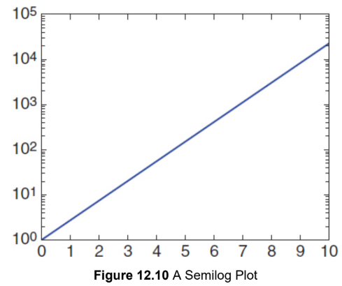
axis ratio

spacing based on a ratio, usually 10, 100, 1000, and so on

Tables

more likely to contain disjointed information than either charts or graphs because they often contain categorical data or experimental results; significant organization is likely to be relevant; should be able to convert it to a rough graph or to a linear equation

Correlation

a connection—direct relationship, inverse relationship, or otherwise—between data

correlation coefficient

number between –1 and +1 that represents the strength and direction of the relationship

+1 = strong positive relationship

–1 = strong negative relationship

0 = no apparent relationship

causation

manipulation of one variable is the reason for an effect in another