Key Concepts in Statistics and Experimental Design

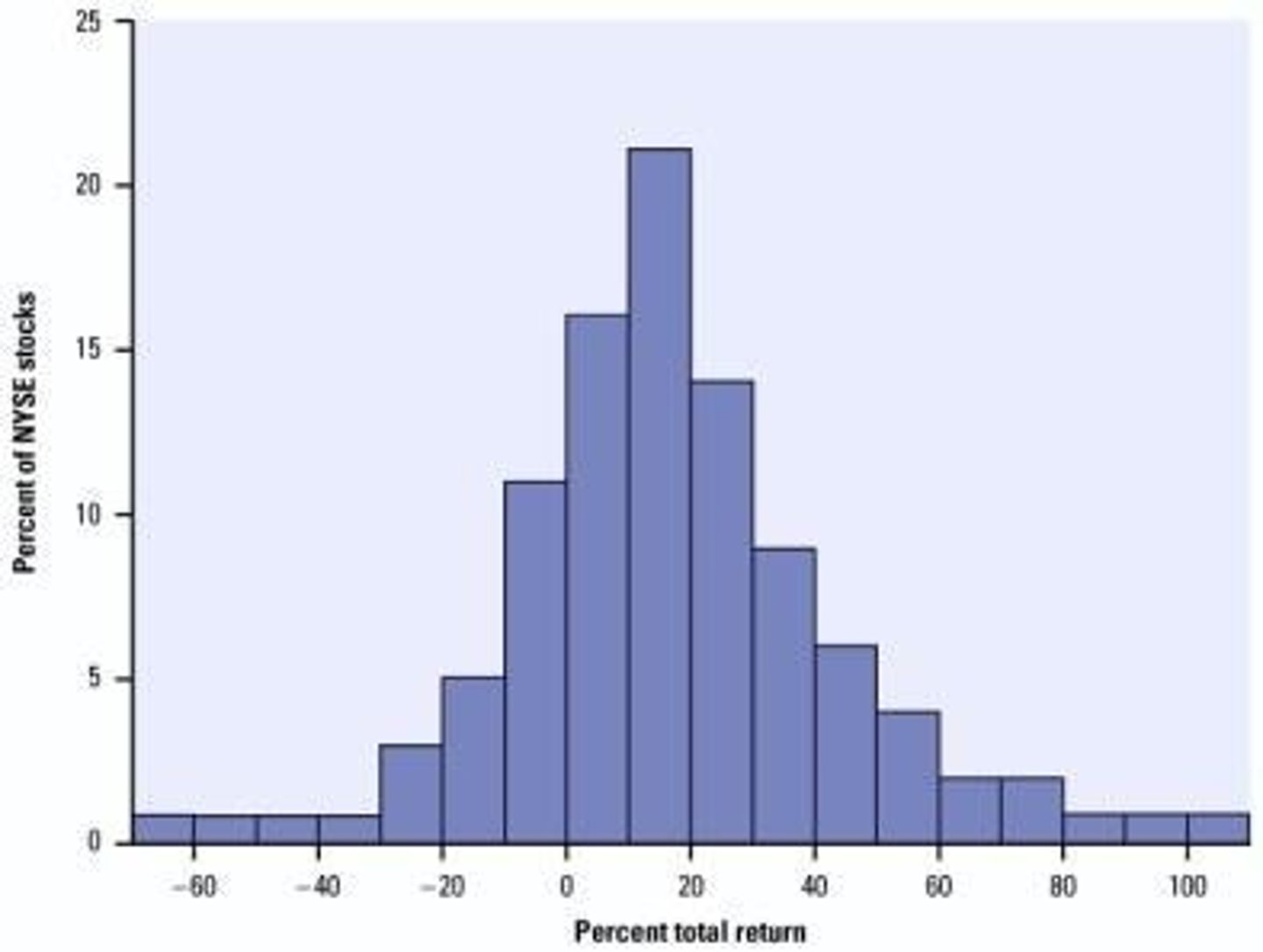
Histogram

fairly symmetrical, unimodal

Linear transformation - Addition

affects center NOT spread; adds to M, Q1, Q3, IQR

IQR

Q3 - Q1

Test for an outlier

1.5(IQR) above Q3 or below Q1

Describing data

describe center, spread, and shape.

5 number summary

or mean and standard deviation when necessary.

Linear transformation - Multiplication

affects both center and spread; multiplies M, Q1, Q3, IQR, σ

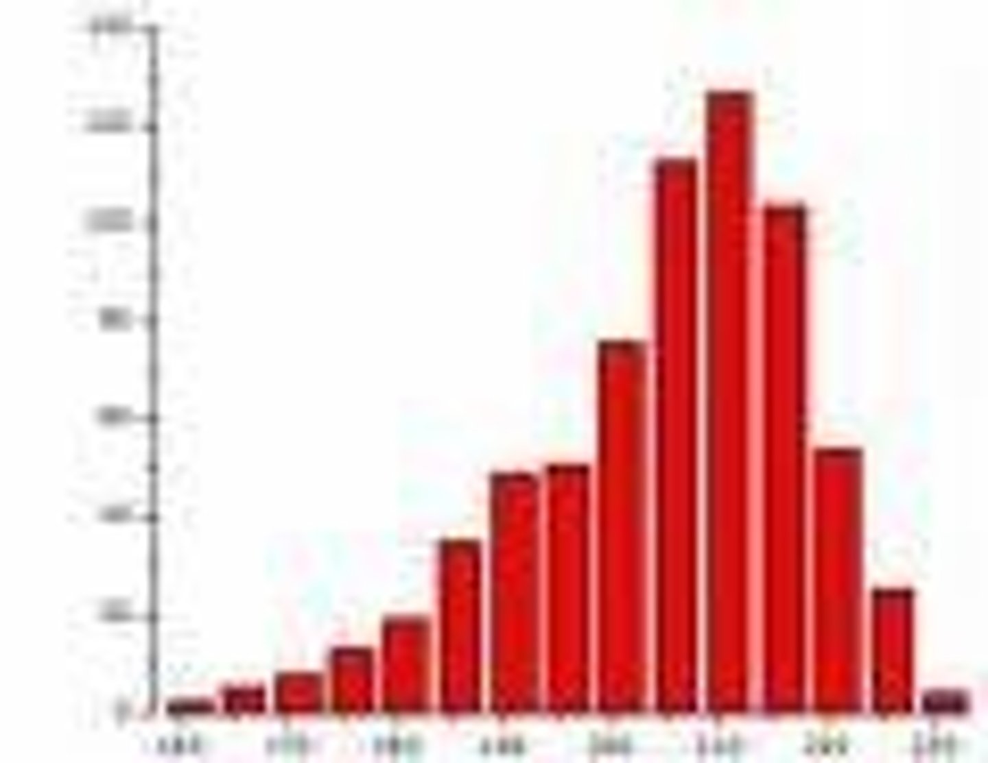
Skewed left

A distribution where the left tail is longer than the right.

Skewed right

A distribution where the right tail is longer than the left.

Ogive

cumulative frequency

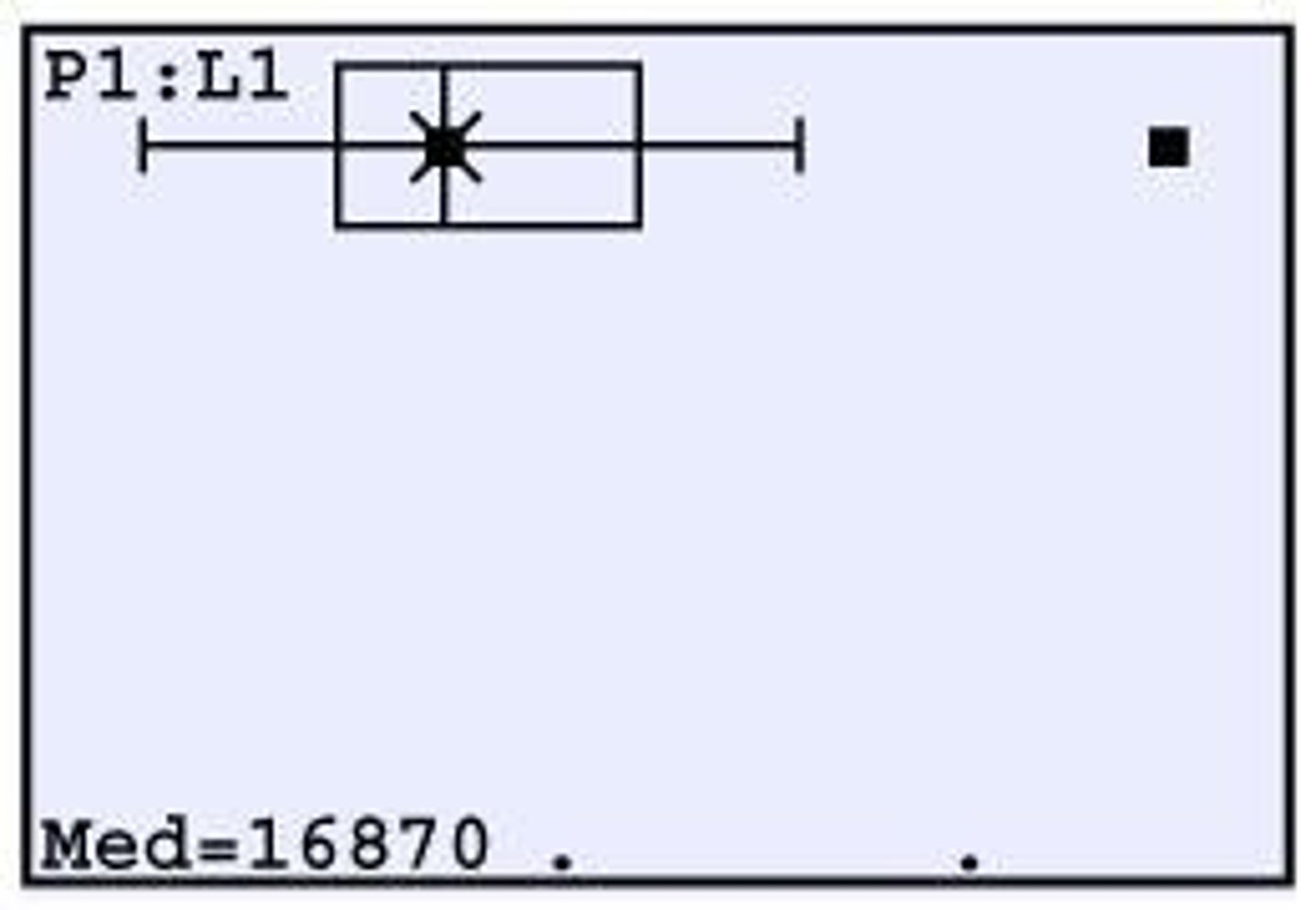
Boxplot

A graphical representation of data that shows the distribution based on a five-number summary.

Stem and leaf

A method of displaying quantitative data in a graphical format.

Normal Probability Plot

A graphical technique for assessing whether or not a data set follows a normal distribution.

r: correlation coefficient

The strength of the linear relationship of data; close to 1 or -1 is very close to linear.

r2: coefficient of determination

How well the model fits the data; close to 1 is a good fit.

80th percentile

Means that 80% of the data is below that observation.

Standard deviation from the mean

HOW MANY STANDARD DEVIATIONS AN OBSERVATION IS FROM THE MEAN

68-95-99.7 Rule for Normality

Describes the percentage of data within one, two, and three standard deviations from the mean.

Exponential Model

y = abx; take log of y

Power Model

y = axb; take log of x and y

Explanatory variables

explain changes in response variables; EV: x, independent; RV: y, dependent.

Lurking Variable

A variable that may influence the relationship between two variables; LV is not among the EV's.

Residual

observed - predicted

Slope of LSRL(b)

rate of change in y for every unit x

y-intercept of LSRL(a)

y when x = 0

Confounding

two variables are confounded when the effects of an RV cannot be distinguished.

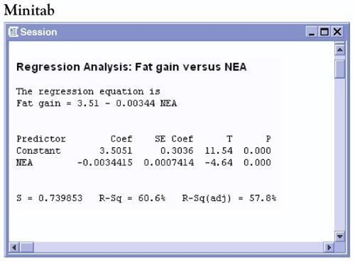
Regression equation

The regression equation is: y = a + bx

Predicted fat gain

Predicted fat gain is 3.5051 kilograms when NEA is zero.

Moderate, negative correlation

r = -0.778; correlation between NEA and fat gain.

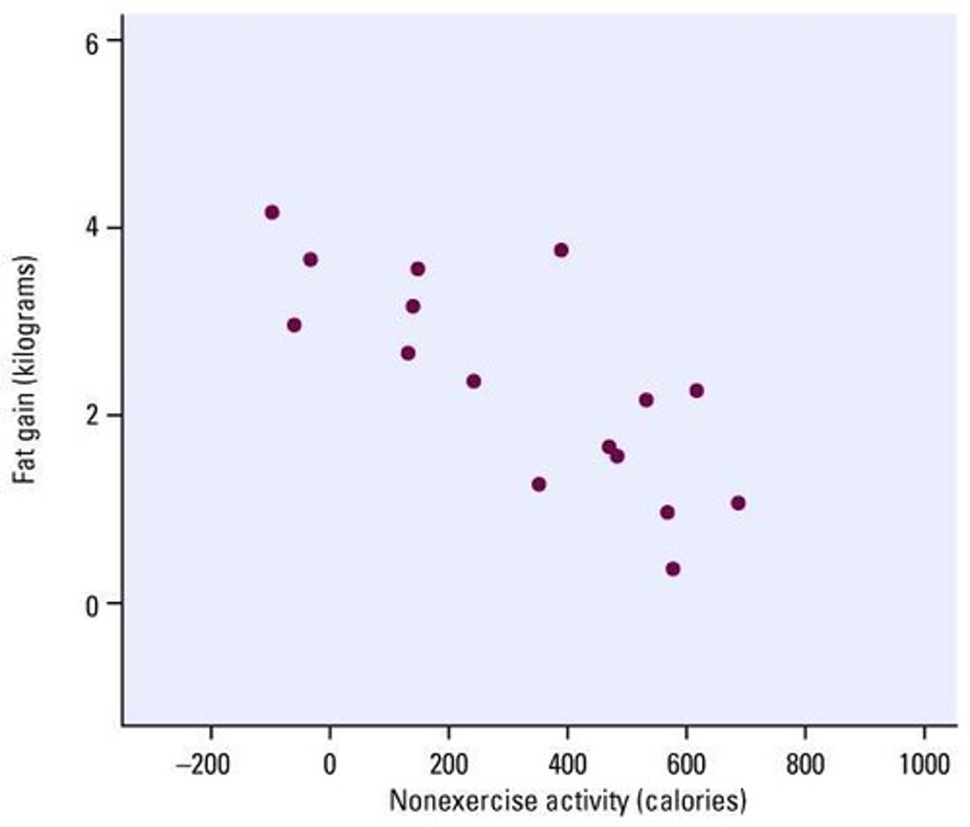
Coefficient of determination

r2 = 0.606; 60.6% of the variation in fat gained is explained by the Least Squares Regression line on NEA.

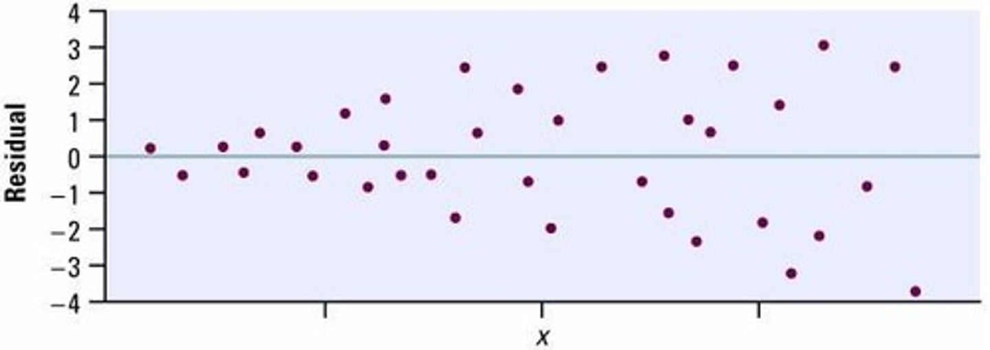
Residual plot

shows that the model is a reasonable fit; there is not a bend or curve.

Extrapolation

Predicting outside the range of our data set.

Confidence interval for the slope

Construct a 95% Confidence interval for the slope of the LSRL of IQ on cry count.

t

A statistic used in regression analysis, with a value of 3.07.

p

The p-value in regression analysis, with a value of 0.004.

s

The standard deviation of the residuals, with a value of 17.50.

Voluntary sample

A sample made up of people who decide for themselves to be in the survey.

Example of voluntary sample

Online poll.

Convenience sample

A sample made up of people who are easy to reach.

Example of convenience sample

Interview people at the mall or in the cafeteria.

Simple random sampling

A method in which all possible samples of n objects are equally likely to occur.

Example of simple random sampling

Assign a number 1-100 to all members of a population of size 100 and select the first 10 without repeats.

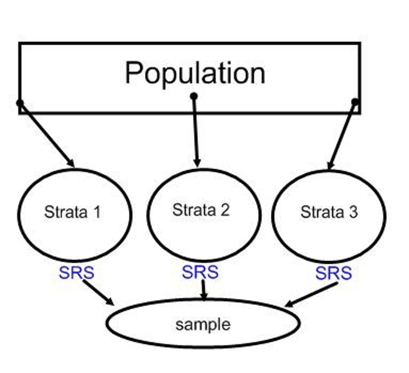
Stratified sampling

A method where the population is divided into groups based on some characteristic, and SRS is taken within each group.

Example of stratified sampling

Dividing the population into groups based on geography and randomly selecting respondents from each stratum.

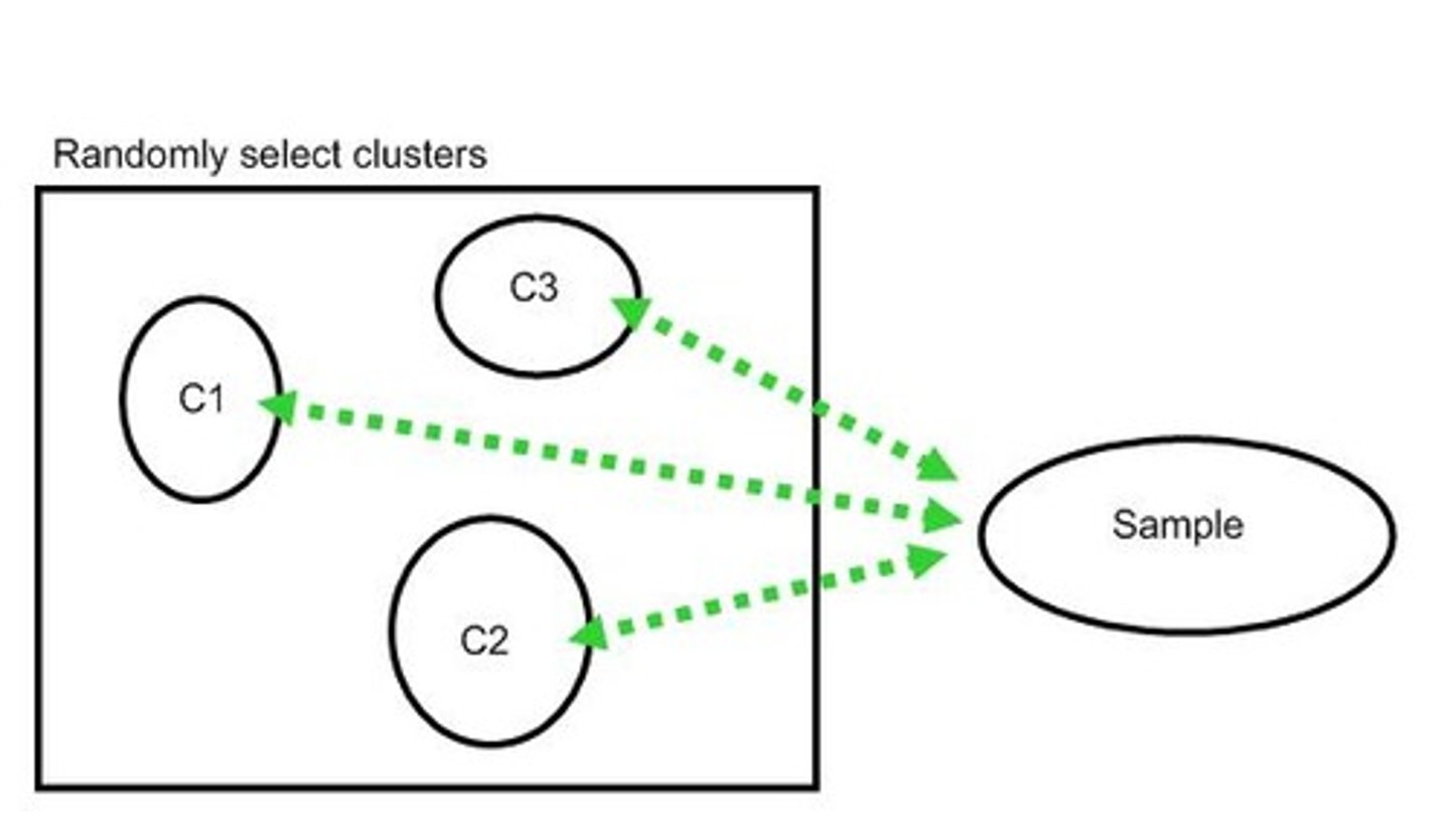
Cluster sampling

A method where every member of the population is assigned to one group, and a sample of clusters is chosen using SRS.

Example of cluster sampling

Randomly choosing high schools in the country and surveying only people in those schools.

Difference between cluster sampling and stratified sampling

Stratified sampling includes subjects from each stratum, while cluster sampling includes subjects only from sampled clusters.

Multistage sampling

A method that uses combinations of different sampling methods.

Example of multistage sampling

Using cluster sampling to choose clusters and then simple random sampling to select subjects from each chosen cluster.

Systematic random sampling

A method where a list of every member of the population is created, and every kth subject is selected.

Example of systematic random sampling

Select every 5th person on a list of the population.

Experimental Unit or Subject

The individuals on which the experiment is done.

Factor

The explanatory variables in the study.

Level

The degree or value of each factor.

Treatment

The condition applied to the subjects.

Control

Steps taken to reduce the effects of other variables, called lurking variables.

Control group

A group that receives no treatment.

Placebo

A fake or dummy treatment.

Blinding

Not telling subjects whether they receive the placebo or the treatment.

Double blinding

Neither the researchers nor the subjects know who gets the treatment or placebo.

Randomization

The practice of using chance methods to assign subjects to treatments.

Replication

The practice of assigning each treatment to many experimental subjects.

Bias

When a method systematically favors one outcome over another.

Completely randomized design

With this design, subjects are randomly assigned to treatments.

Randomized block design

The experimenter divides subjects into subgroups called blocks. Then, subjects within each block are randomly assigned to treatment conditions.

Matched pairs design

A special case of the randomized block design used when the experiment has only two treatment conditions; subjects can be grouped into pairs based on some blocking variable.

Simple Random Sample

Every group of n objects has an equal chance of being selected.

Stratified Random Sampling

Break population into strata (groups) then take an SRS of each group.

Cluster Sampling

Randomly select clusters then take all members in the cluster as the sample.

Systematic Random Sampling

Select a sample using a system, like selecting every third subject.

Counting Principle

If Trial 1 has a ways, Trial 2 has b ways, and Trial 3 has c ways, then there are a x b x c ways to do all three.

Independent events

A and B are independent if the outcome of one does not affect the other.

Mutually Exclusive events

A and B are disjoint or mutually exclusive if they have no events in common.

Conditional Probability

For Conditional Probability use a TREE DIAGRAM.

P(A)

0

P(B)

0

P(A ∩B)

0

P(A U B)

0.3 + 0.5 - 0.2 = 0.6

P(A|B)

0.2/0.5 = 2/5

P(B|A)

0.2 /0.3 = 2/3

Binomial Probability

Look for x out of n trials with success or failure, fixed n, independent observations, and p is the same for all observations.

P(X=3)

Exactly 3, use binompdf(n,p,3).

P(X≤ 3)

At most 3, use binomcdf(n,p,3) (Does 3,2,1,0).

P(X≥3)

At least 3 is 1 - P(X≤2), use 1 - binomcdf(n,p,2).

Normal Approximation of Binomial

For np ≥ 10 and n(1-p) ≥ 10, the X is approx N(np, σ²).

Geometric Probability

Look for the number of trials until the first success.

Discrete Random Variable

Has a countable number of possible events (e.g., Heads or tails, each .5).

Continuous Random Variable

Takes all values in an interval (e.g., normal curve is continuous).

Law of large numbers

As n becomes very large, the sample mean will converge to the expected value.

P(X=n)

p(1-p)^(n-1) for trials until first success.

P(X > n)

(1 - p)^n = 1 - P(X ≤ n).

Sampling distribution

The distribution of all values of the statistic in all possible samples of the same size from the population.

Central Limit Theorem

As n becomes very large the sampling distribution for is approximately NORMAL.

Use (n ≥ 30) for CLT

Indicates the sample size required to apply the Central Limit Theorem.

Low Bias

Predicts the center well.

High Bias

Does not predict center well.

Low Variability

Not spread out.

High Variability

Is very spread out.

Type I Error

Reject the null hypothesis when it is actually True.

Type II Error

Fail to reject the null hypothesis when it is False.