Midterm 1 Coding

Virtually resampling 1000 times with size 50

virtual_resampled_means <- pennies_sample %>%

rep_sample_n(size = 50, replace = TRUE, reps = 1000) %>%

group_by(replicate) %>%

summarize(mean_year = mean(year))

virtual_resampled_means

• takes 1000 resamples, calculates the mean for each of them

virtual_resampled_means <- pennies_sample %>%

rep_sample_n(size = 50, replace = TRUE, reps = 1000) %>%

group_by(replicate) %>%

summarize(mean_year = mean(year))

virtual_resampled_means

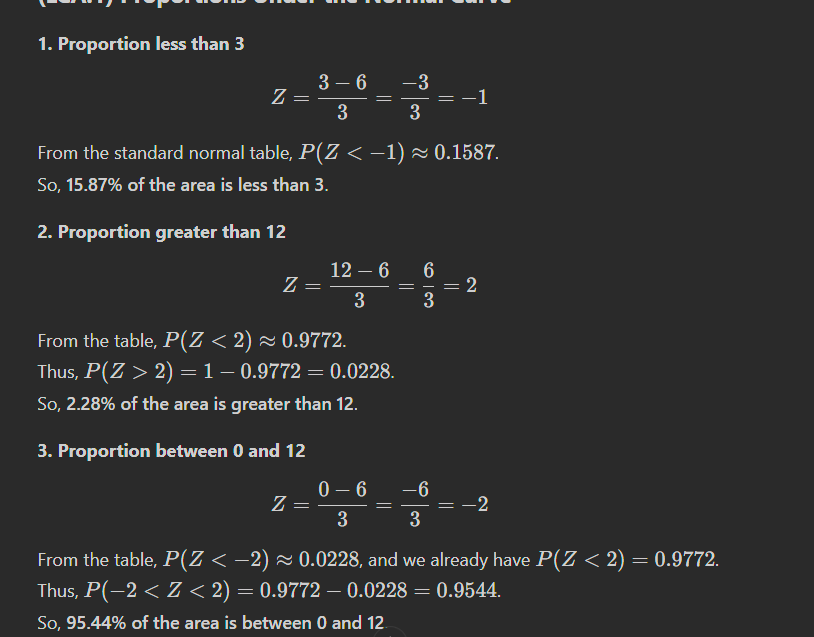
Say you have a normal distribution with mean μ=6 and standard deviation σ=3.

(LCA.1) What proportion of the area under the normal curve is less than 3? Greater than 12? Between 0 and 12?

(LCA.2) What is the 2.5th percentile of the area under the normal curve? The 97.5th percentile? The 100th percentile?

• use z score to get distance, then convert the score to a percentile

  • pnorm(zscore) → percentile

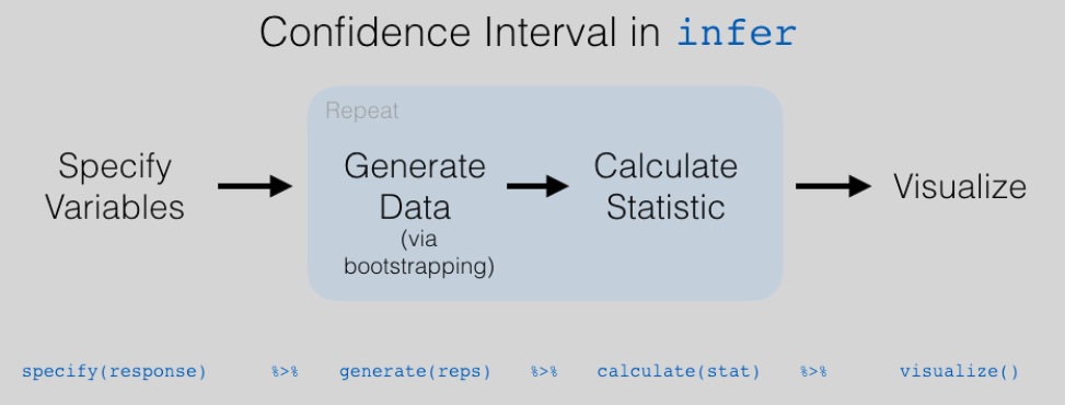
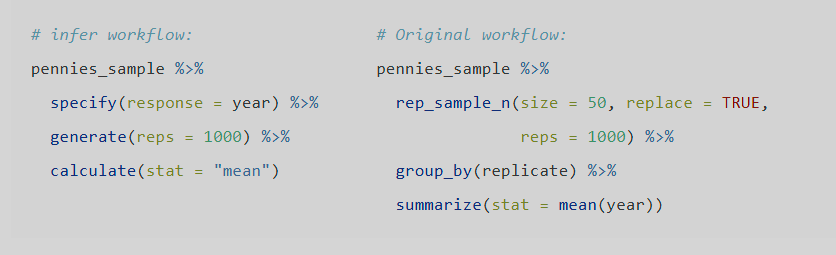
infer package

1. functionally equivalent to rep_sample_n

1. specify: the variable you are interested in

2. generate: generate the samples (equivalent to rep_sample_n)

3. calculate: calculate the statistic you are interested in (equivalent to group by and summarize)

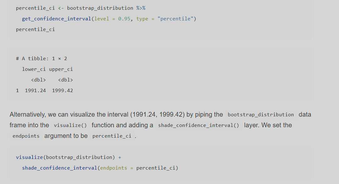
4. get_confidence_interval (equivalent to summarize and quantile)

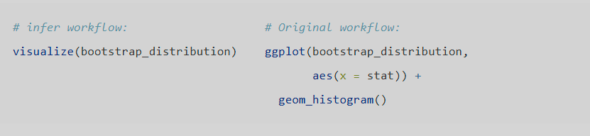
Visualizing infer results

Percentile method

Testing success of a confidence interval

sample_1_bootstrap <- bowl_sample_1 %>%

specify(response = color, success = "red") %>%

generate(reps = 1000, type = "bootstrap") %>%

calculate(stat = "prop")

sample_1_bootstrap

Visualization

percentile_ci_1 <- sample_1_bootstrap %>%

get_confidence_interval(level = 0.95, type = "percentile")

percentile_ci_1

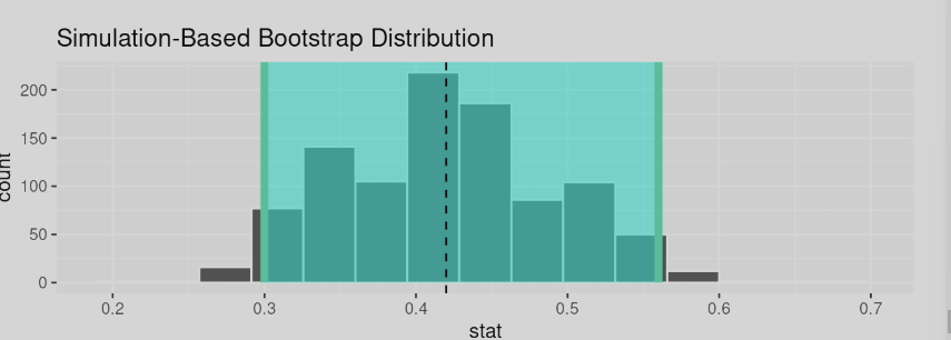
sample_1_bootstrap %>%

visualize(bins = 15) +

shade_confidence_interval(endpoints = percentile_ci_1) +

geom_vline(xintercept = 0.42, linetype = "dashed")

Pnorm and Qnorm

Probability

1. this is the area belwo the curve

2. u =10, std = 3 and want area below 11.5

   1. pnrom( 11.5, mean = 10, sd = sqrt(3))

   2. automatically takes the area to the left of the specified pthis is the oint

Quantile

1. From the area we know, need the value on the axis

2. qnorm(0.69, mean = 10, sd = sqrt(3))

Value of curve? → dnorm(x,std

CLT equations

• Sample values are independent

  • Generally, if your sample size is greater than 10% of the population size, there will be a violation of independence.

  • if you go beyond 10% of population size you wil lbe in trouble since sampling with replacement violates independence

• Sample size must be large enough.

  • For means:

    • no universal guideline for how big 𝑛n should be

    • but, usually sample >30 are big enough to get a reasonable approximation (not guaranteed!)

      • no way for you to check and also larger sample size the better

  • For proportions:

    • check 𝑛×𝑝≥10n×p≥10 and 𝑛×(1−𝑝)≥10

    • if these conditions hold you are good for propotion

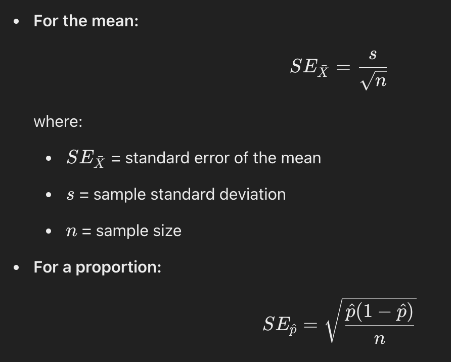
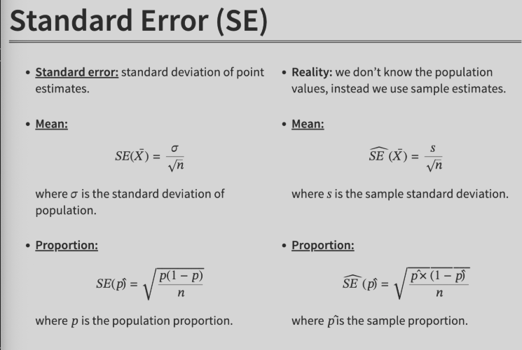
Standard error equations

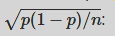
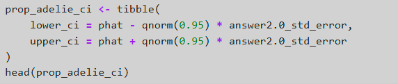
How to optain a CI for proportion

• it is mean of the proportion- qnorm of the CI+1/2 of the uncovered area *sqrt(p(1-p)/n

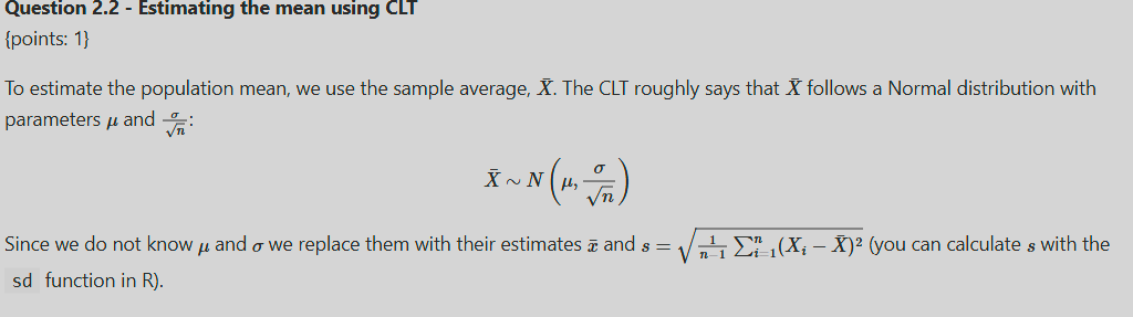
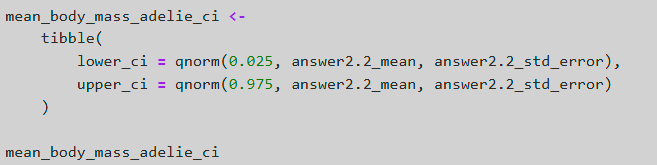
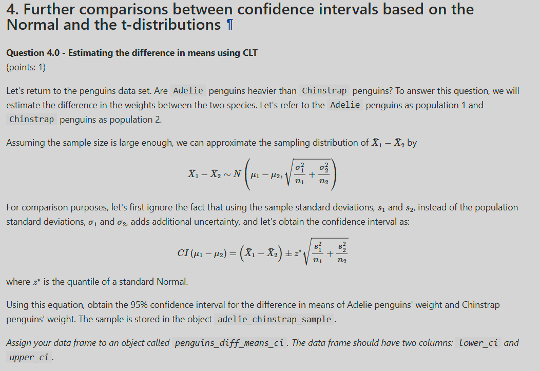
Estimating the mean using CLT

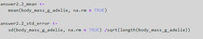
Calculating CI for the mean

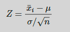
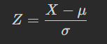
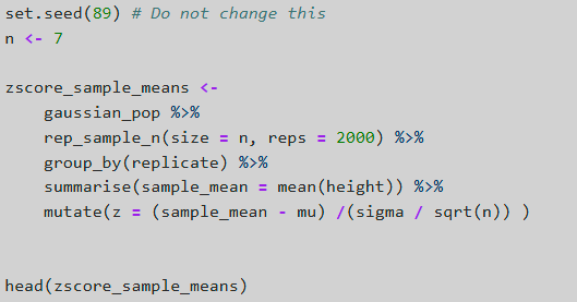
Z score

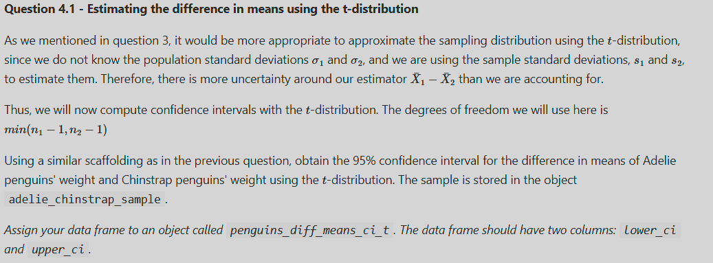
qt vs qnorm

The reason qt() is needed for small-sample means is not just because there are "more variables" but because the sample standard deviation itself is a random variable

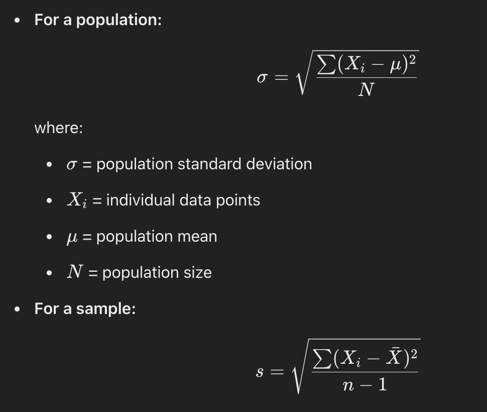
Standard deviation equation for a population and for a sample

Standard error for a sample mean and proportion