Statistics 2 Lecture 11

Models in statistics

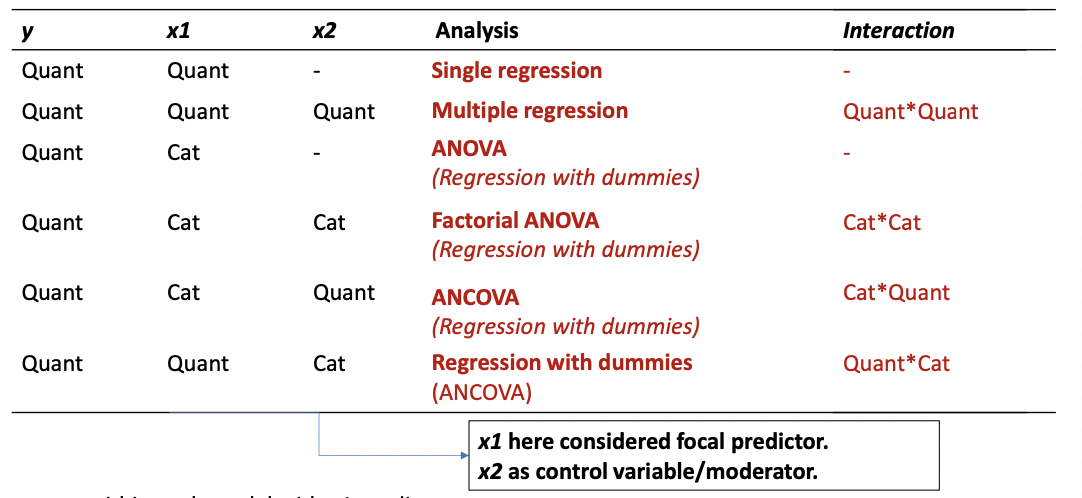
GLM parameters: quantitative predictors for multiple regression with interactions

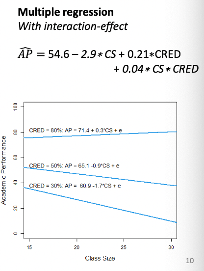
• y = a + b1*x1 + b2*x2 + b3*x1*x2

• a: expected y when all x are 0

• b1: expected change in y when x1 increases with 1 unit and x2 is 0

• b2: expected change in y when x2 increases with 1 unit and x1 is 0

• b3:

  • x1 as focal predictor → predicted change in the effect of x1 when x2 increases with 1 unit

  • x2 as focal predictor → predicted change in the effect of x2 when x1 increases with 1 unit

• → Slopes differ depending on second predictor

GLM parameters: quantitative predictors for multiple regression without interactions

• y = a + b1*x1 + b2*x2
  a: expected y when all x are 0

• b1: expected change in y when x1 increases with 1 unit and x2 [all other x] stay constant

• b2 : expected change in y when x2 increases with 1 unit and x1 [all other x] stay constant

• → Slopes do not differ, they are constant at different levels of second predictor

GLM with categorical predictors: Dummy variables

• Dummy-variables allow us to include categorical predictors in a regression model: 𝒚 =𝑎+𝑏1∗𝑧1+𝑏2∗𝑧2+ ...+𝑏𝑔−1 ∗𝑧𝑔−1

• Each dummy-variable (𝑧𝑖) indicates if an observation belongs to that specific group.

  • 𝑧𝑖 = 1 if participant belongs to group i

  • 𝑧𝑖 = 0 if participant does not belong to group i

• We need 𝑔 − 1 dummy variables to identify all groups

• For 3 groups thus 3-1 = 2 dummy-variables required, for example:

  • 𝒛𝟏 = 1 for participants in group 1

  • 𝒛𝟏 = 0 for participants in group 2 and group 3

  • 𝒛𝟐 = 1 for participants in group 2

  • 𝒛𝟐 = 0 for participants in group 1 and group 3

  • Group with 0 on each dummy variable is called the ‘reference category’

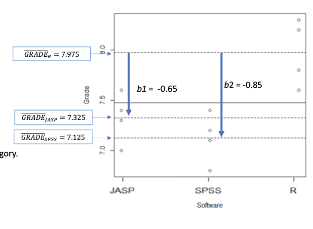
Example Dummy varaibles

• 𝒛𝟏 = 1 for students using JASP, 0 for all other students 𝒛𝟐 = 1 for students using SPSS, 0 for all other students

• Regression-equation (estimated with least squares; OLS):

  Grade = a + b1 z1 + b2 * z2 =

  7.975 − 0.650 ∗ 𝐽𝐴𝑆𝑃 − 0.850 ∗ 𝑆𝑃𝑆𝑆

• 𝑧1 = 0 and 𝑧2 = 0: Grade = 7.975 − 0.650 ∗ 0 − 0.850 ∗ 0 = 7.975 → Mean GradeR

• 𝑧1 = 1 and 𝑧2 = 0: Grade = 7.975 − 0.650 ∗ 1 − 0.850 ∗ 0 = 7.325 → Mean GradeJASP

• 𝑧1 = 0 and 𝑧2 = 1:Grade = 7.975 − 0.650 ∗ 0 − 0.850 ∗ 1 = 7.125 → Mean GradeR

Interpretation coefficients dummy-variables

• Intercept a: Group mean of the reference category

• Slope b: Deviation of group mean 𝑦ഥ from the mean of the reference category. 𝑖

• In the example:

  • a = 7.975: GradeR

  • b1 = −0.650: GradeJASP - GradeR

  • b2 = −0.850: GradeSPSS - GradeR

Dummy-coding for multiple factors

• When we include multiple factors in our model, we need to create dummy variables for both factors:

• For Factor A (software; 3 levels), for example:

  • 𝒛𝟏 = 1 for students using JASP, 0 for all other students

  • 𝒛𝟐 = 1 for students using SPSS, 0 for all other students

  • → R as reference category

• For Factor B (course; 2 levels):

  • 𝒘𝟏 = 1 for STAT1 students, 0 for all other students

  • → STAT 2 as reference category

• And dummy variables for their interaction terms:

  • By multiplying the dummies of both factors (not within factors!!):

  • 𝒛𝟏* 𝒘𝟏 = 1 for students using JASP in STAT1, 0 for all other students

  • 𝒛𝟐 * 𝒘𝟏= 1 for students using SPSS in STAT1, 0 for all other students

• We can use these dummy-variables in a regression model to predict y

• 𝒚 = 𝑎 + 𝑏1 ∗ 𝑧1 + 𝑏2 ∗ 𝑧2 + 𝑏3 ∗ 𝑤1 + 𝑏4 ∗ 𝑧1 ∗ 𝑤1 + 𝑏5 ∗ 𝑧2 ∗ 𝑤1

New Data Example

• Does Statistics 1 grade predict motivation, and does this association depend on the software students use? →Always start with testing the interaction-effect.

• Based on this question, variables have the following roles:

  • motivation: Criterion (outcome) variable

  • stat1Grade: Focal predictor

  • software: moderator

• Model with main- and interaction-effects of statistic 1 grade (Stat1Grade) and software type (software) on motivation

• 𝒎𝒐𝒕𝒊𝒗𝒂𝒕𝒊𝒐𝒏 = -2.224 + 0.634*grade – 1.010*R – 0.086*SPSS + 0.136*grade*R + 0.004*grade*SPSS

• Completing the equation helps interpreting interaction-effects: What is the ‘effect’ of statistics 1 grades on motivation among R-users?

  • 𝒎𝒐𝒕𝒊𝒗𝒂𝒕𝒊𝒐𝒏 = -2.224 + 0.634*grade – 1.010*1 – 0.086*0 +

    0.136*grade*1 + 0.004*grade*0 =
    -2.224 + 0.634*grade – 1.010*1 + 0.136*grade*1 = -3.234 + 0.770*grade (answer = 0.770)

• What is the ‘effect’ of statistics 1 grades on motivation among JASP-users?

• What is the ‘effect’ of statistics 1 grades on motivation among SPSS-users?

Reduced model

• Model is a reduced version of complete model when it includes the same but less parameters than the complete model→Models are nested

• Said differently: Reduced model includes a subset of the effects of the complete model.

• Hypotheses for model comparison:

  • H0: All parameters in complete model that are not present in reduced model = 0 → one model is not explaining is better than another one

  • HA: At least one of the parameters in which the models differ ≠ 0.

(Explained) variation in the regression model

• Quality of predictions in (multiple) regression models:

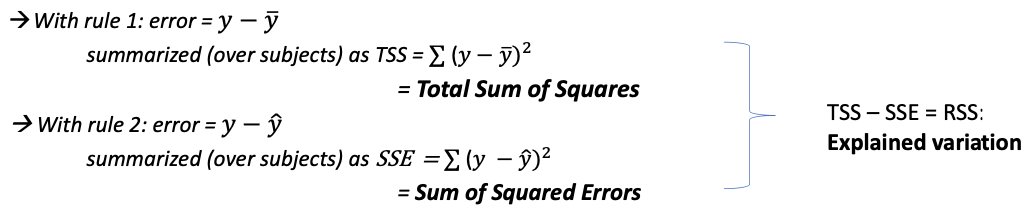
• Rule 1:
  When we predict 𝑦 without any x:
  →The sample mean 𝒚ഥ is the best prediction

• Rule 2:

  When we predict 𝑦 with any x:
  →The prediction equation 𝒚ෝ = 𝒂 + 𝒃𝟏𝒙𝟏 + 𝒃𝟐𝒙𝟐 + ... + 𝒃𝒌𝒙𝒌 is

  the best prediction.

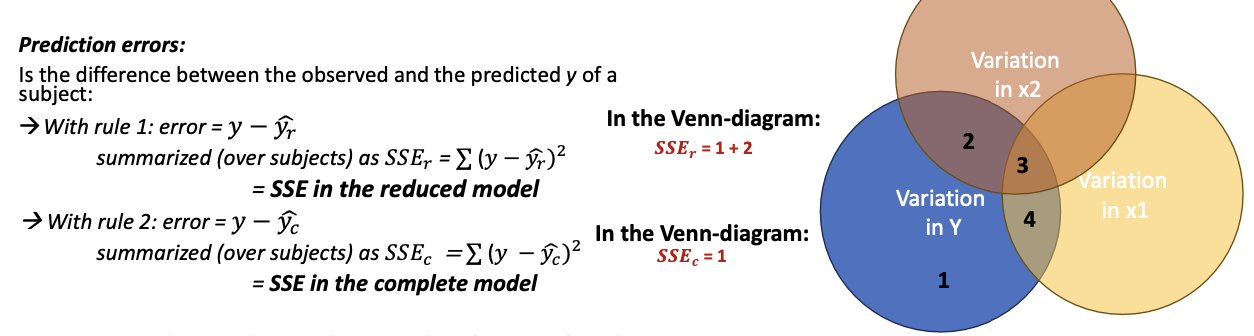
• Prediction errors:

• Is the difference between the observed and the predicted y of a subject

Familiar rules applied to Model C and Model R

• Rule 1:

  When we predict 𝑦 with x1:
  → The prediction equation 𝒚ෞ = 𝒂 + 𝒃 𝒙 makes the best prediction.

• Rule 2:

  When we predict 𝑦 with x1 and x2:
  →The prediction equation 𝒚ෞ = 𝒂 + 𝒃 𝒙 + 𝒃 𝒙 makes the best prediction.

• Prediction errors:

• Is the difference between the observed and the predicted y of a subject

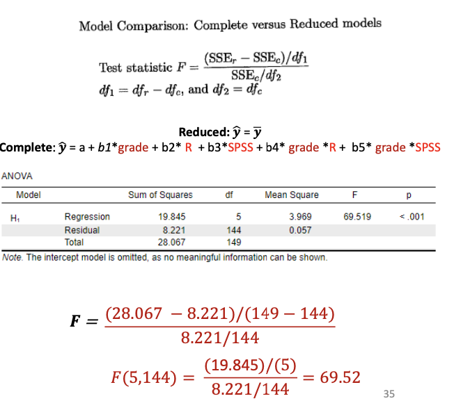
The F-test for model comparison

• Compares the residual sums of squares (SSE) of:

  • Complete model

  • Reduced model

• Test the explanatory power of the extra predictors in the complete model.

• Models can be extended with more parameters as long as the reduced model is a simplified version → The model should be nested

• 𝐝𝒇𝟏 = 𝑑𝑓 – 𝑑𝑓 →difference in number of b coefficients between models 𝑟𝑐

• 𝒅𝒇𝟐 = 𝑑𝑓 → degrees of freedom after estimating all parameters

• For example:

  • Complete model: 𝑦 = 𝑎 + 𝑏1𝑥1 + 𝑏2𝑥2

  • Reduced model: 𝑦 = 𝑎 + 𝑏1𝑥1

• F-test significant? Reject H0, Conclude that the additional parameter is significant: here, b2 ≠ 0.

• F-test not significant? No evidence to reject the H0

Example: SS and df2 complete and reduced model

• Unexplained variation reduced model?

  • IF reduced model has no predictors: SSEr = SST → Thus SSEr = 28.067

  • df2 reduced model?

  • IF model has no predictors: N-k-1 = N-0-1 = N-1 149 (N – 1)

• Unexplained variation complete model?

  • SSE𝑐 = 8.221

  • df2 complete model?

  • 144 (N – (k +1))

• Difference unexplained variation reduced and complete model?

  • SSEr – SSE𝑐 = 28.067 – 8.221 = 19.845

  • →SSR! Because reduced model did not contain predictors.

  • Difference in df2? 149 - 144 = 5 (k!)