CFA Vol-1: Quantitative Methods

Coefficient b0 is the

“intercept,” representing the expected

value of Y if all independent variables are zero

There are five main assumptions underlying multiple regression models

(1) linearity,

(2) homoskedasticity, (The variance of the regression residuals is the same for all observations. /expected value of the eror term is equal to zero, we must evaluate whether the variance

of the regression residuals is constant for all observations; to compare scatterplot of the regression residuals versus the predicted values)

(3) independence of errors,

(4) normality (is about the distribution/shape of residuals overal)

(5) independence of independent variables (to compare scatterplot comparing the values of two of the independent variables)

5a. Independent variables are not random.

5b. There is no exact linear relation between two or more of the independent

variables or combinations of the independent variables

If, however, the dependent variable is discrete—for example, an indicator variable such as whether a company is a takeover target or not a takeover target—then, as we shall see, the model may be estimated as

A logistic regression.

P value <5% =>>

Variable is significant at the 5% significance level

Coefficient determination (R^2, R-squared): (definition)

is a measure of the goodness of fit of an estimated regression to the data. (How much variability are explained in this regression model)

Coefficient determination (R^2, R-squared): (formula)

Problems with using R2 in multiple regression include the following:

i) The R2 cannot provide information on whether the coefficients are statistically significant.

ii) The R2 cannot provide information on whether there are biases in the estimated coefficients and predictions.

iii) The R2 cannot tell whether the model fit is good. A good model may have a low R2, as in many asset-pricing models, and a bad model may have a high R2 due to overfitting and biases in the model.

Overfitting of a regression model is a situation in which the model is

too complex, meaning there may be too many independent variables relative to the number of observations in the sample.

adjusted R2 (formula)

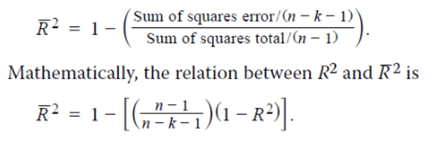
Linear F statistic formula: (standart)

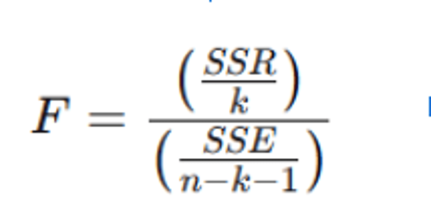
We test the role of the jointly omitted variables using the following F-distributed test statistic (formula)

(where q is the number of restrictions, meaning the number of variables omitted in the restricted model compared to the unrestricted model)

Adjusted R2 (better higher or lower)

Higher

AIC (Akaike`s information criterion and BIC (Schwarz`s Bayesian infirmation criterion (better higher or lower)

Lower

AIC (Akaike`s information criterion

Indicates for predictive models

BIC

Goodnes if fit if desired

Omiited variable (as failure)

Onemli seviyede etki edebilecek bir parametreyi modele dahil etmemem sonucu diger parametrenin oneminin gereksiz artmasi (biased olmasi) ve onemli parametrenin missing olmasi:

The Breusch–Pagan (BP) (definition)

test is widely used in financial analysis to diagnose potential

conditional heteroskedasticity and is best understood via the three-step process.

Eğer P-değeri < 0.05 ise → %5 anlamlılık düzeyinde heteroskedastisite vardır.

Eğer P-değeri ≥ 0.05 ise → homoskedastisite varsayımı sağlanmıştır.

The Breusch–Pagan (BP) test (formula)

nR^2

Serial correlation

Zaman serisi regresyonlarında, hata terimlerinin birbirine bağımlı olması durumudur. Yani bugünkü hata, dünkü hatayla bağlantılıysa serial correlation var demektir.

Testing for Serial Correlation (two tests)

Durbin Watson Test and Breusch-Godfrey test

The most common “fix” for a regression with significant serial correlation is to...

adjust the coefficient standard errors to account for the serial correlation.

Breusch-Godfrey test

is more robust because it can detect autocorrelation up to a pre-designated order p. If the BG value exceed the critical value than there is serial correlation.

Durbin Watson Test:

Limiting because it applies only to testing for the first-order serial correlation. (Eğer hata terimleri daha yüksek dereceden gecikmelerle bağlıysa (örneğin utu_tut​ ile ut−2u_{t-2}ut−2​ veya ut−3u_{t-3}ut−3​) → DW testi bunu yakalayamaz.)

VIOLATIONS OF REGRESSION ASSUMPTIONS: MULTICOLLINEARITY

Bağımsız değişkenlerin (X’lerin) birbirleriyle aşırı derecede ilişkili (korrelasyonlu) olmasıdır.

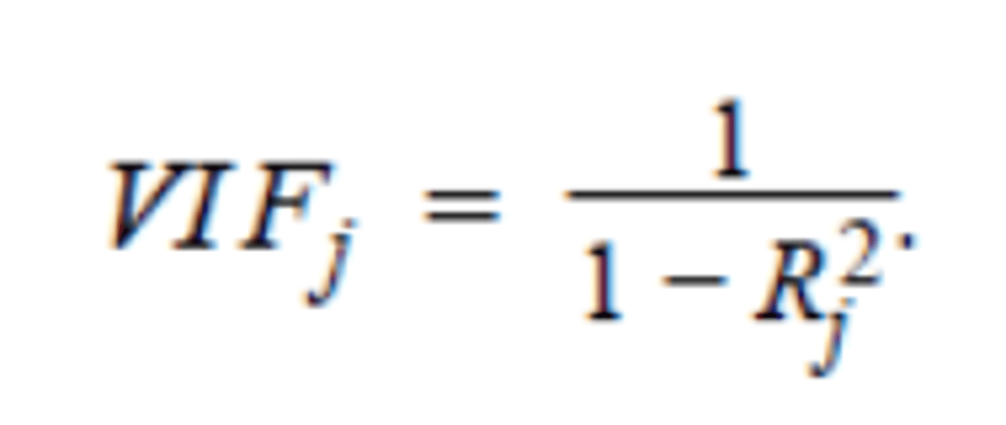
Variance inflation factor (VIF) to quantify multicollinearity

Issues (formula)

VIFj > 5 warrants further investigation of the given independent variable.

VIFj >10 indicates serious multicollinearity requiring correction.

Possible solutions to multicollinearity include

excluding one or more of the regression variables,

using a different proxy for one of the variables,

and

increasing the sample size.

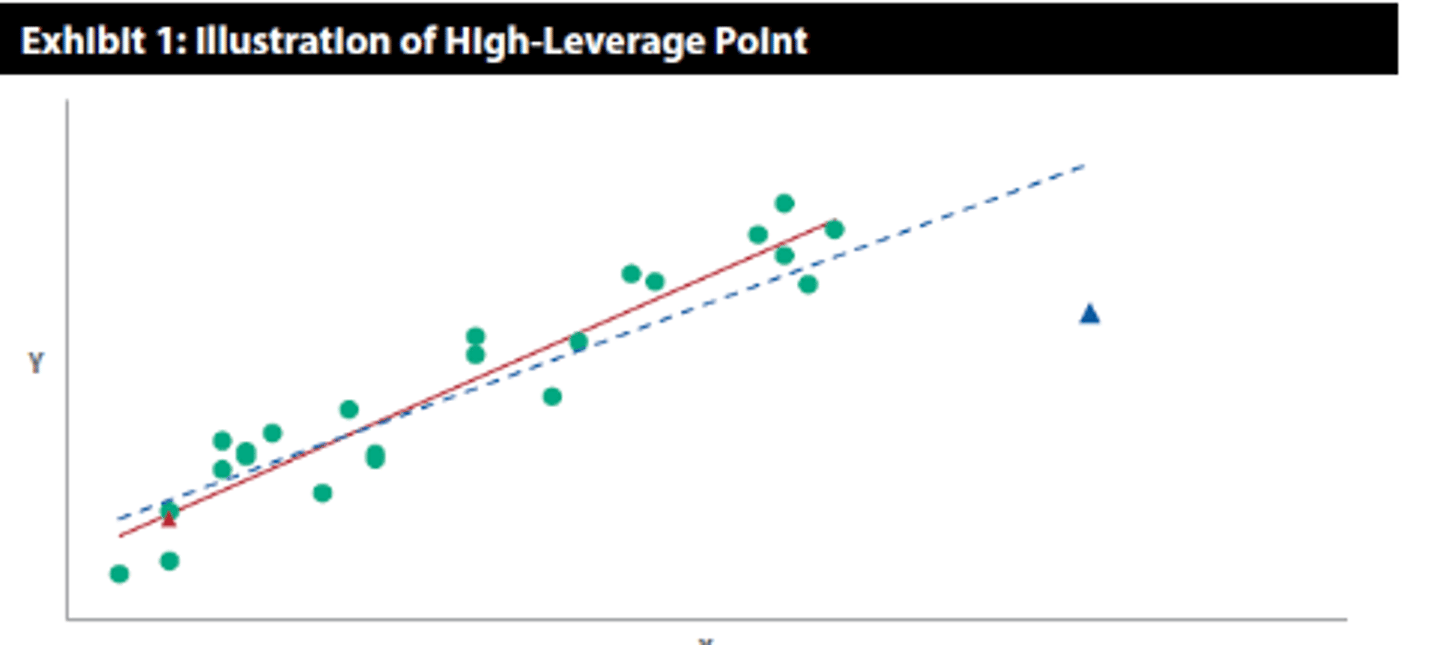
A high-leverage point

A data point having an extreme value of an independent

Variable (X valuesinin Y ye gore fazla olmasi)

An outlier

A data point having an extreme value of the dependent variable

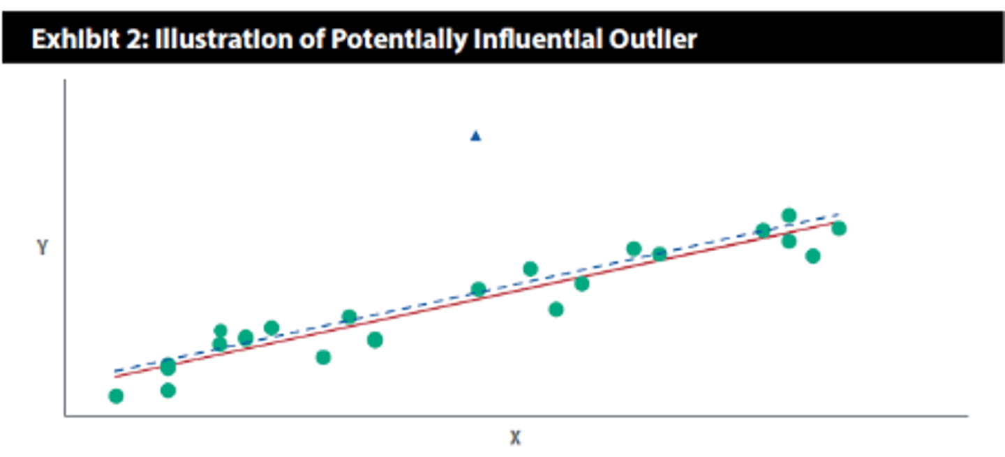
A high-leverage point can be identified using a measure called

Leverage (hii). Leverage is a value between 0 and 1, and the higher the leverage, the more distant the observation’s value is from the variable’s mean

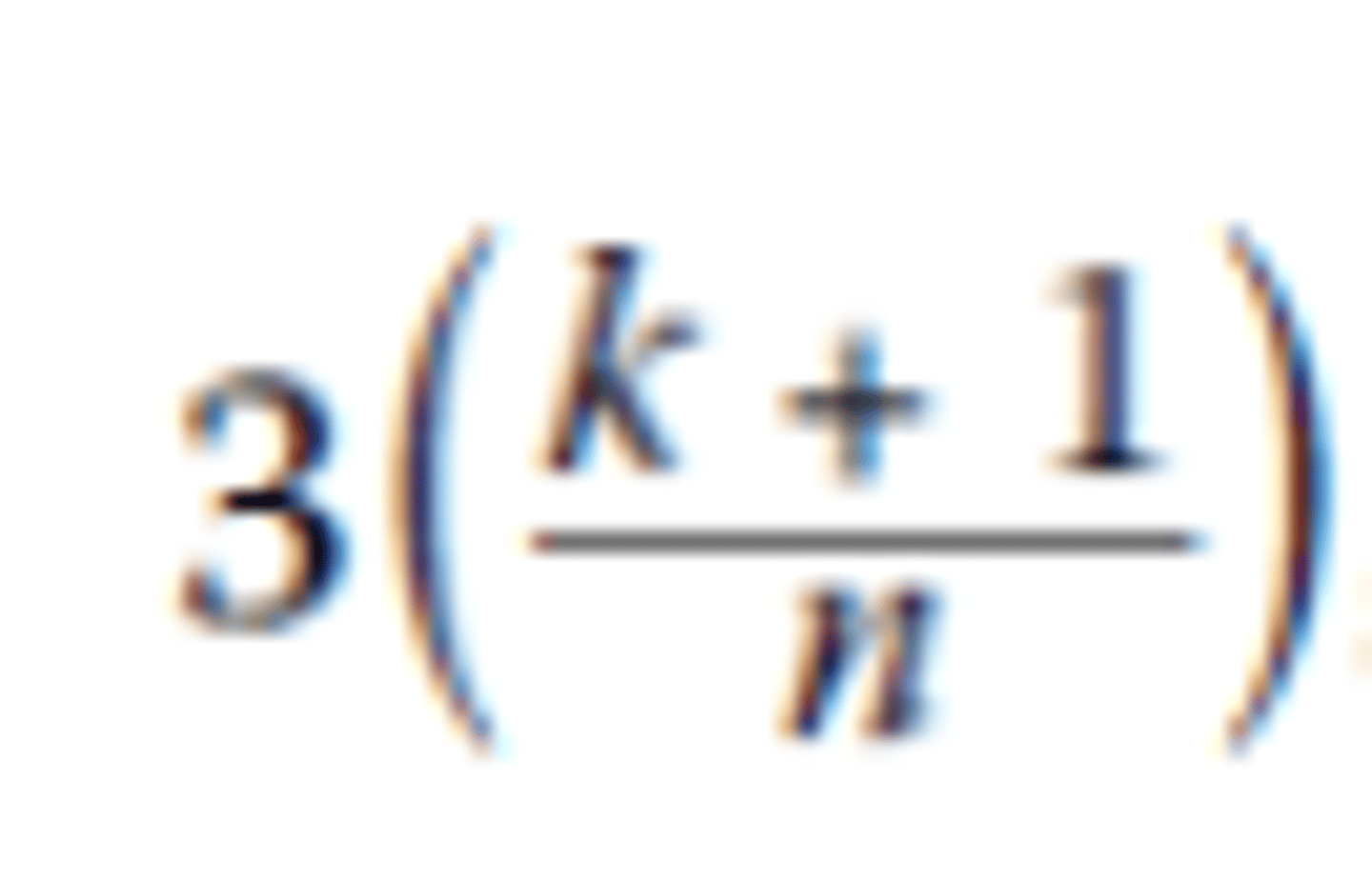
As for identifying outliers, observations with unusual dependent variable values, the preferred method is to use

Studentized residuals.

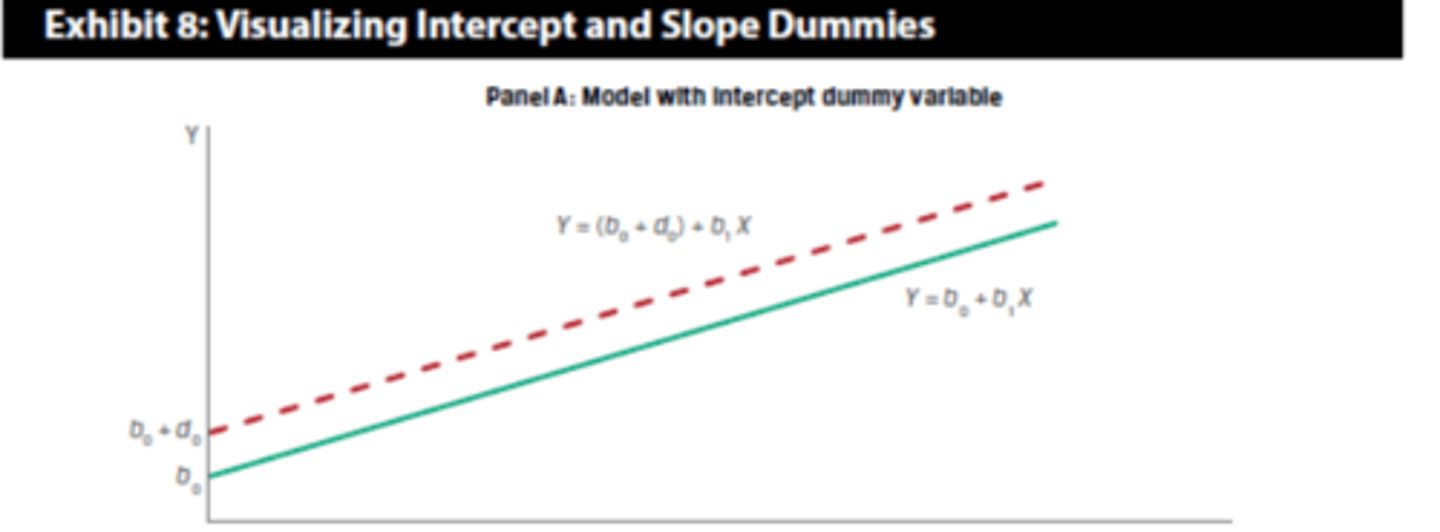
Intercept dummy (D)

yi=b0+d0D+b1Xi+ei

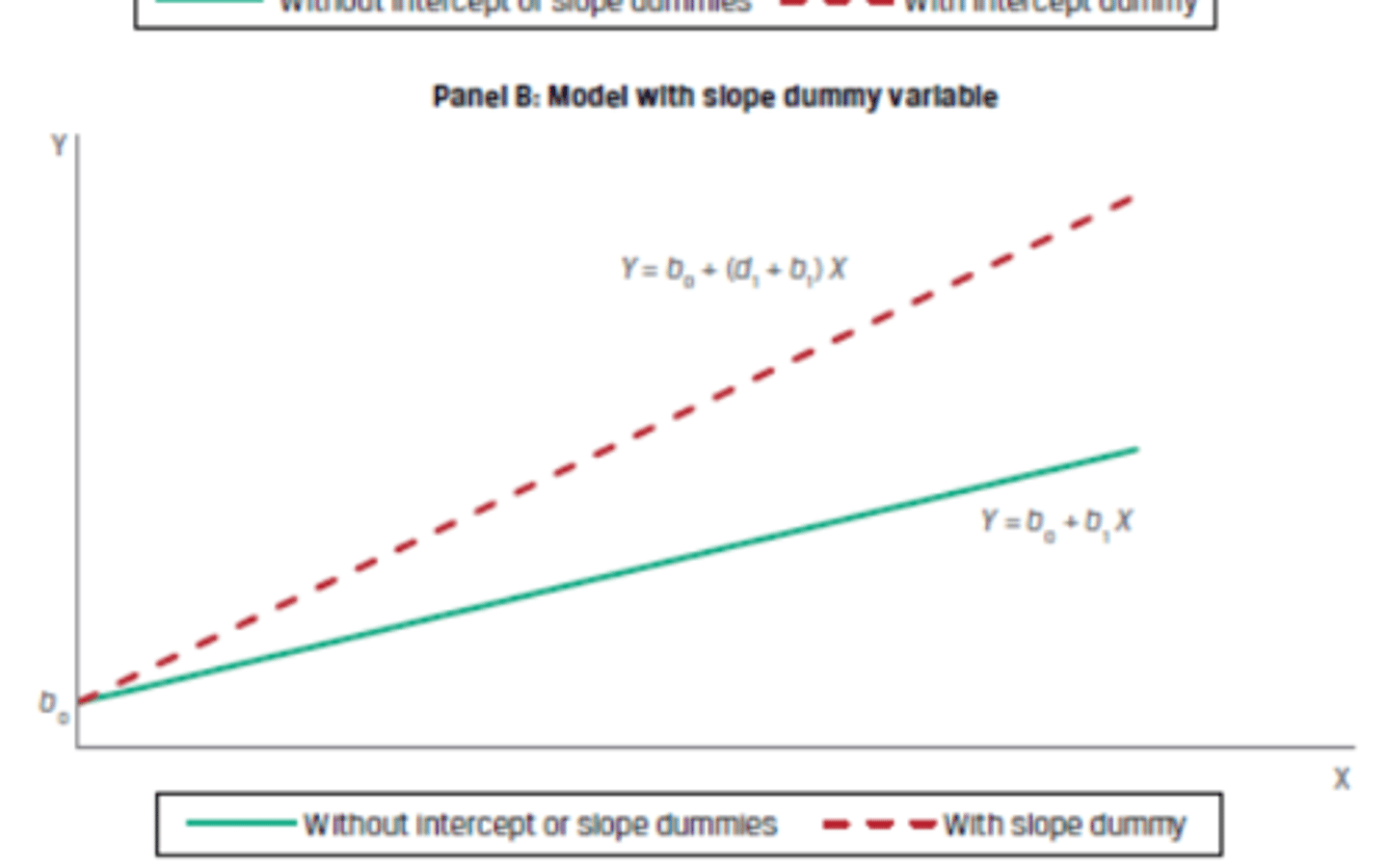
A Slope dummy

yi= b0+b1Xi+d1DiXi+ei

Non-linear transformation to the probability of bankruptcy

For example, if the probability of a company going bankrupt is 0.75 and P/(1 − P)

is 0.75/(1 − 0.75) = 3, the odds of bankruptcy are 3 to 1.

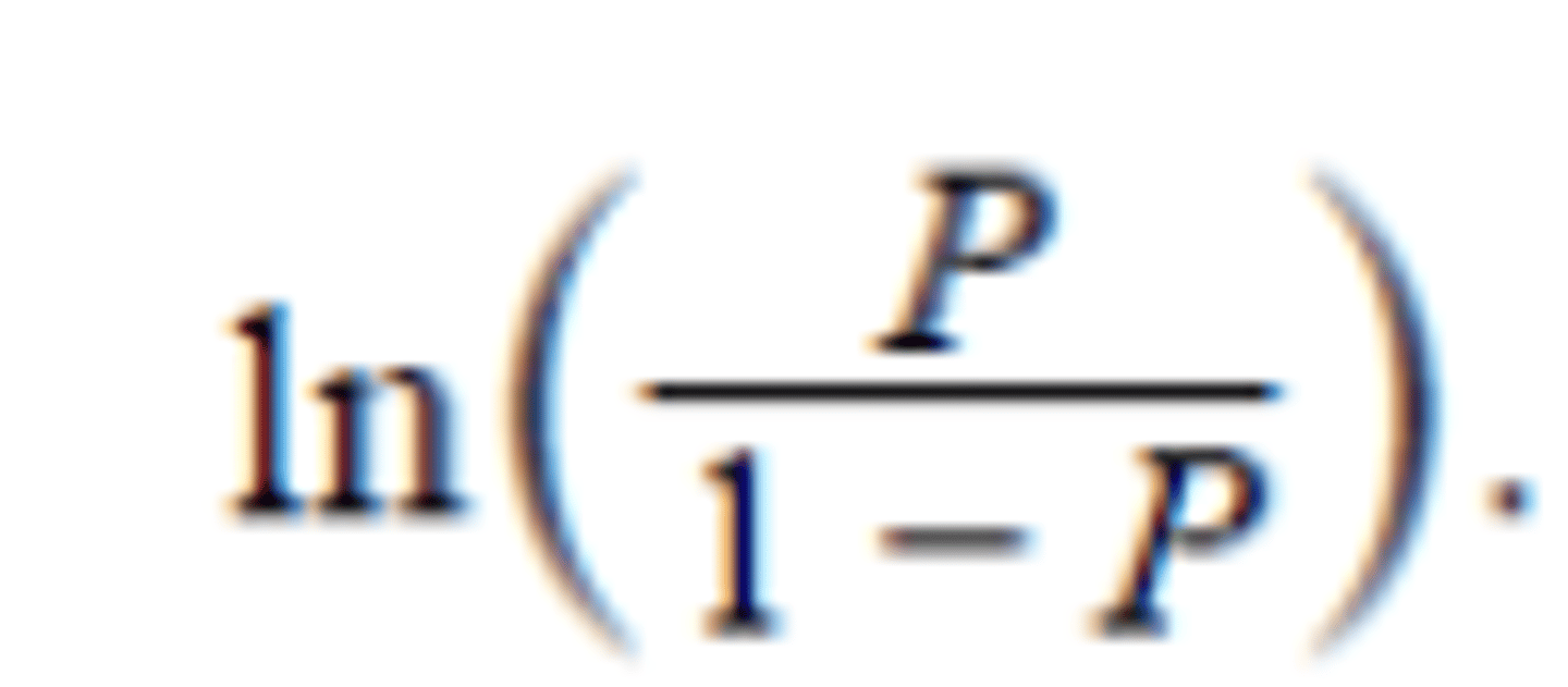
Logistic regression (logit)

Uses the logistic transformation of the event probability

(P) into the log odds, as the dependent variable

The likelihood ratio (LR) test

is a method to assess the fit of logistic regression models and is based on the log-likelihood metric that describes the fit to the data. (Log likelihood da sifira yakin olan daha iyi fit demek.)

DW ≈ 2 ise ,

DW < 2 ise,

DW > 2 ise

DW ≈ 2 ise her şey yolunda demek. DW < 2 ise pozitif serisel korelasyon var. DW > 2 ise negatif serisel korelasyon var. (Douglas Wilson)

Pozitif serisel korelasyon

Bu şu demek: model geçmişte yaptığı hataları “tekrar ediyor”, dolayısıyla daha iyi model kurulabilir.

Çözüm → AR (veya ARIMA gibi) modeller

AR modeli..

..zaman serisinin bugünkü değerini kendi geçmiş değerlerine bakarak tahmin etmeye çalışır.

Bir zaman serisinin covariance-stationary (kovaryans-durağan) olması, zamanla değişmeyen istatistiksel ozelliklere sahip olması demektir. Bu tür seriler, zaman serisi analizinde (özellikle AR, MA, ARMA modellerinde) temel varsayım olarak kabul edilir.

Covariance-stationary üc kosulu

i) Sabit Ortalama (Constant Mean) Serinin beklenen değeri zamanla değişmez. Örnek: Ortalama enflasyon %5 civarında sabit kalıyorsa → uygun.;

ii) Sabit Varyans (Constant Variance) Eğer veride dalgalanmalar zamanla büyüyorsa (örneğin kriz dönemlerinde patlıyorsa) → bu koşul sağlanmaz.

iii) Sabit Kovaryans / Otokovaryans (Constant Autocovariance) Yani serinin herhangi bir geçmiş değerle olan ilişkisi zamanın kendisine değil, sadece ne kadar geride olduğuna bağlıdır.

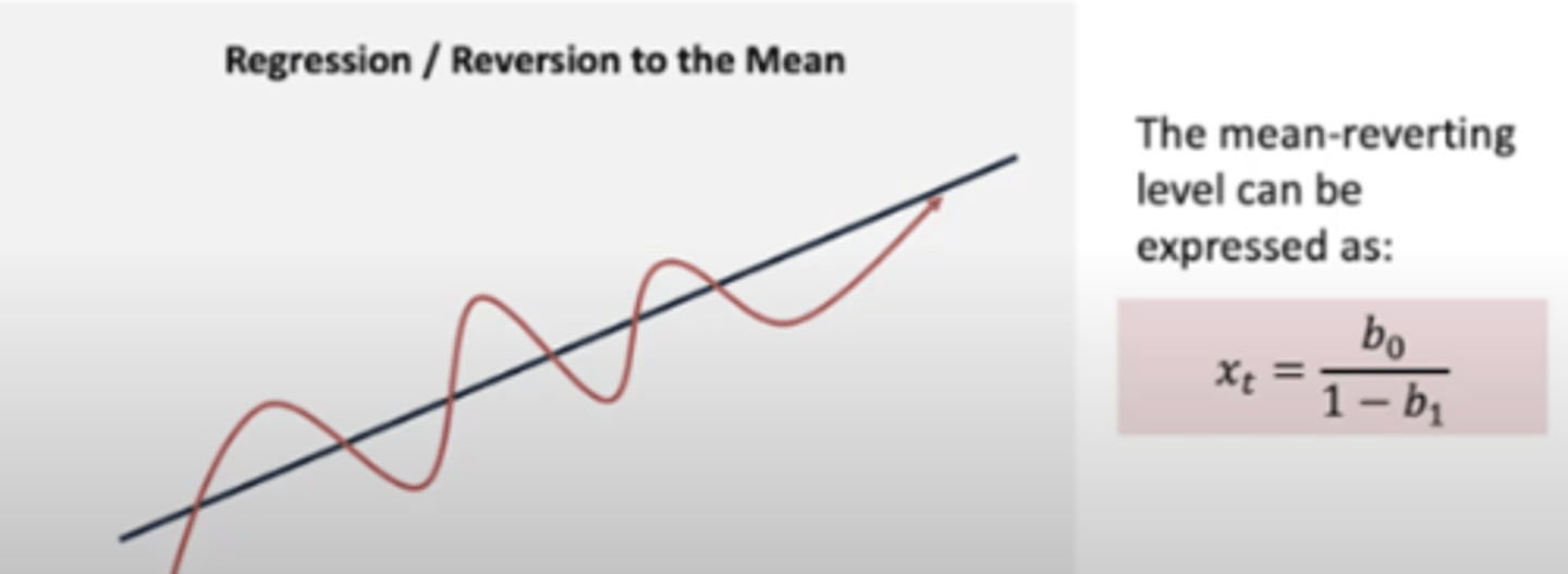
Bir zaman serisi mean-reverting ise

Zamanla ortalama değerine geri dönme eğilimi gösterir.

We compare the out-of-sample forecasting performance of forecasting

models by comparing their

Root mean squared error (RMSE),

The model with the smallest RMSE is judged the

most accurate.

INSTABILITY OF REGRESSION COEFFICIENTS

Regresyon katsayılarının zamanla değişmesi veya farklı dönemlerde tutarsız sonuçlar vermesi durumuna denir.

Yani model bugün çalışıyor, ama 6 ay sonra aynı veri tipiyle aynı sonucu vermiyor. Katsayılar sabit değil → kararsız, model güvensiz hale gelir.

Ne zaman ortaya cikar:

i) Zaman serisi duragan degilse (ortalama varyans, covaryans zamanla degisiyor,

ii) structural change (pandemi, regülasyon degisikligi, sirket birlesmesi,

iii) model spesifikasyon hatalari

Random Walk

Bir zaman serisinin tamamen rastgele ve sistemsiz bir şekilde hareket ettiği durumdur.

Her yeni değer, bir önceki değerin üstüne bir rastgele hata eklenerek oluşur.

(previous period plus an unpredictable random error)

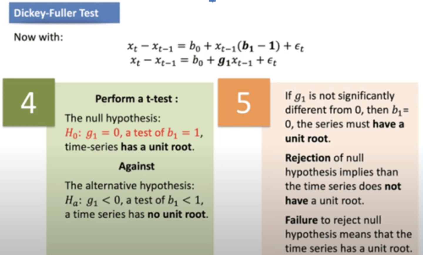
Bir zaman serisinin durağan (stationary) olup olmadığını anlamak için

unit root testi yapılır.

Eğer seride unit root varsa, bu seri non-stationary dir. Yani ortalaması, varyansı zamanla değişir → tahmin yapmak tehlikeli hale gelir.

By definition, all random walks, with or without a drift term, have unit roots.

Dickey and Fuller (1979) developed a regression-based unit root test

AR modeli (Autoregressive - Otoregresif)

bir degiskenin bugunkü degeri, kendi gecmis degerine dayanarak tahmin eder.

Yani: bugün yaşananlar, dünkü beklenmeyen şeylerin etkisiyle oluşmuş olabilir.

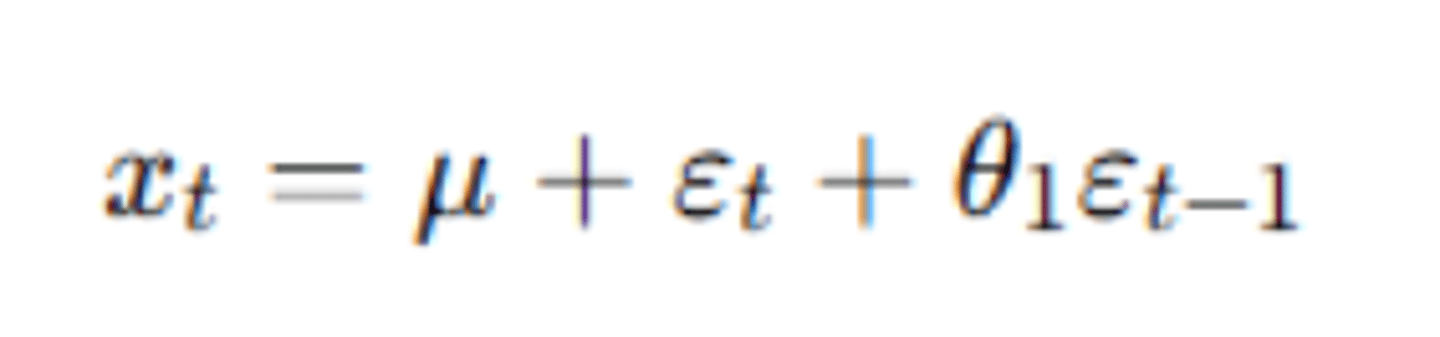
MA (Moving average)

modeli bugunkü deger gecmis hata terimlerine göre modellenir.

ARMA Modeli (AR + MA)

hem gecmis degerler hem de gecmis soklar bugunu etkiler.

ARCH MODELLERİ (Autoregressive Conditional Heteroskedasticity)

hata terimlerinin zamanla degistigi modellerdir; yani volatilitenin de bir modeli vardir.

GARCH MODELLERİ

Hem geçmiş volatiliteyi hem de geçmiş hataları kullanır. ARCH modelinin gelişmiş versiyonudur.

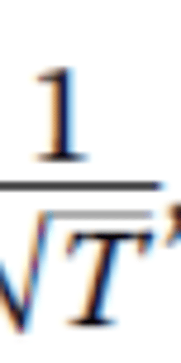
The standard error of the autocorrelations (formula)

Machine learning is broadly divided into three distinct classes of techniques

Supervised learning

Unsupervised learning

Deep learning

Bias error (By Machine learnin)

Algorithms with erroneous assumptions produce high bias with poor approximation, causing underfitting and high in-sample error.

Variance error (By Machine learnin)

or how much the model’s results change in response to new data from validation and test samples.

Unstable models pick up noise and produce high variance, causing overfitting and high out-of-sample error.

Two common methods are used to reduce overfitting

(1) preventing the algorithm from getting too complex during selection and training, which requires estimating an overfitting penalty,

(2) proper data sampling achieved by using cross-validation, a technique for estimating out-of-sample error directly by determining the error in validation samples.

k-fold cross-validation

Veri seti k eşit parçaya ayrılır. Model k kere eğitilir/test edilir, her seferinde farklı bir parça test verisi olur. Sonuçlar ortalanır.

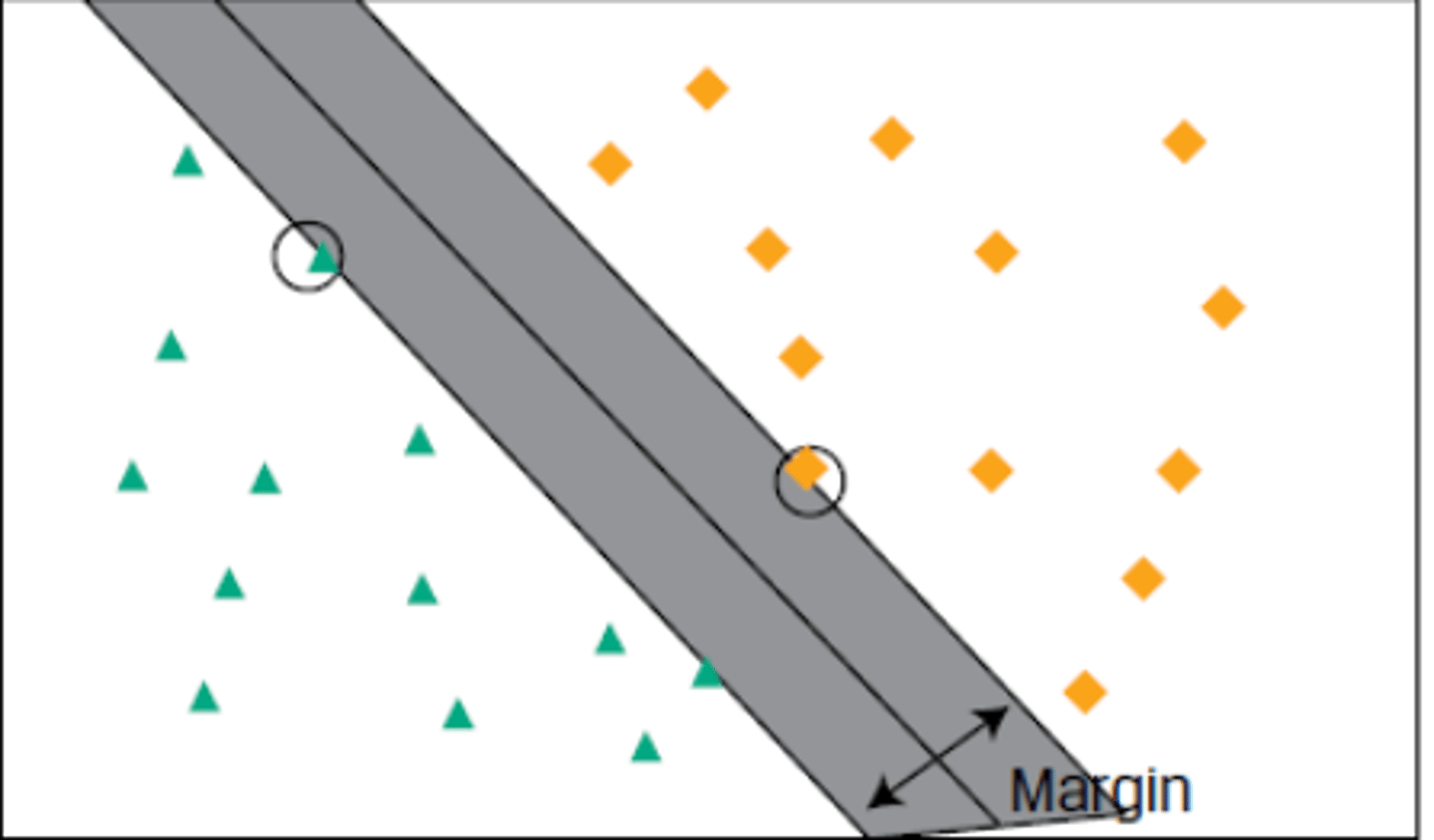
SUPPORT VECTOR MACHINE (SVM)

is a linear classifier that determines the hyperplane that optimally separates the observations into two sets of data points.

K-nearest neighbor (KNN)

is a supervised learning technique used most often for classification and sometimes for regression.

The idea is to classify a new observation by finding similarities (“nearness”) between this new observation and the existing data.

Classification and regression tree (CART)

is another common supervised machine learning technique that can be applied to predict either a categorical target variable, producing a classification tree, or a continuous target variable, producing a regression tree.

CART is commonly applied to binary classification or regression.

Ensemble learning can be divided into two main categories:

(1) aggregation of heterogeneous learners (i.e., different types of algorithms combined with a voting classifier) or

(2) aggregation of homogeneous learners (i.e., a combination of the same algorithm using different training data that are based, for example, on a bootstrap aggregating, or bagging, technique, as discussed later).

Bootstrap aggregating (or bagging)

is a technique whereby the original training dataset is used to generate n new training datasets or bags of data.

Each new bag of data is generated by random sampling with replacement from the initial training set. The algorithm can now be trained on n independent datasets that will generate n new models.

RANDOM FOREST NEDİR

Elindeki veriyi alır, rastgele küçük parçalar oluşturur. Her parça için bir karar ağacı eğitir. Yeni veri geldiğinde: Her ağaç ayrı ayrı tahmin yapar. En çok çıkan tahmin → sonuç olur (oy çokluğu).

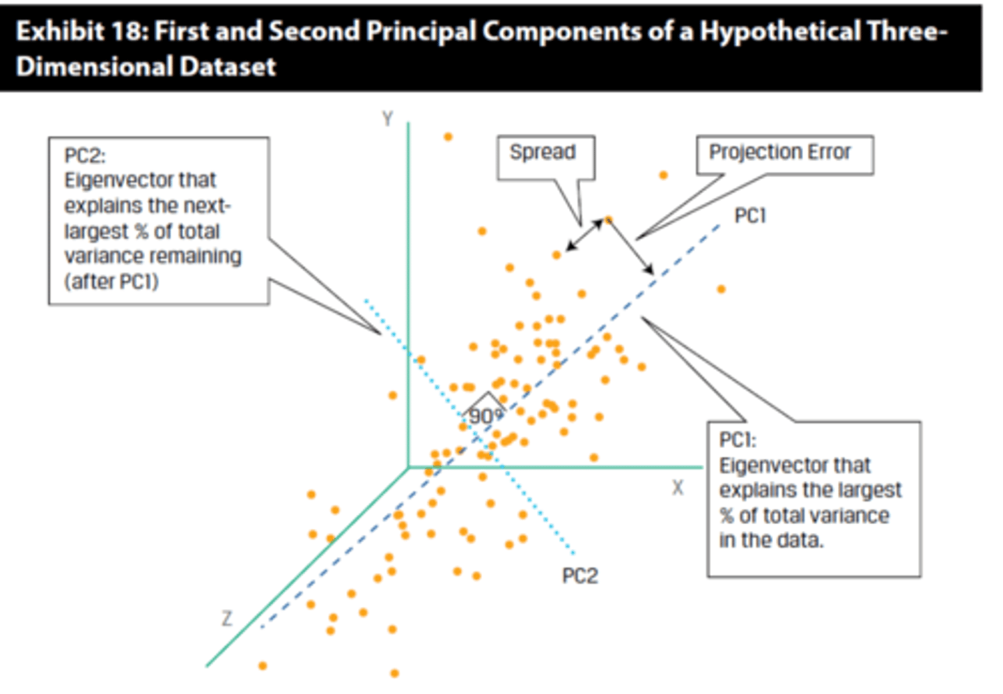
Principal components analysis (PCA)

is used to summarize or transform highly correlated features of data into a few main, uncorrelated composite variables.

Amacı, yüksek derecede ilişkili (correlated) özelliklere sahip bir veri setini, daha az sayıda, birbirleriyle ilişkisiz (uncorrelated) bileşik değişkenlerle özetlemek veya dönüştürmektir.

Özvektörler (Eigenvectors):

Orijinal özelliklerin doğrusal kombinasyonları olan yeni, karşılıklı olarak ilişkisiz bileşik değişkenleri tanımlar. Her özvektör bir yönü temsil eder.

Özdeğerler (Eigenvalues):

Her özvektörle ilişkilidir ve başlangıç verisindeki toplam varyasyonun ne kadarını açıkladığını gösterir.

The main drawback of PCA

is that since the principal components are combinations of the dataset’s initial features, they typically cannot be easily labeled or directly interpreted by the analyst. (BLACK BOX)

K-MEANS CLUSTERING

küme içi uzaklıkları minimize etmeyi ve kümeler arası uzaklıkları maksimize etmeyi hedefleyerek tekrarlayan bir süreç izler.

Agglomerative clustering (or bottom-up hierarchical clustering)

begins with each observation being treated as its own cluster. Then, the algorithm finds the two closest clusters, defined by some measure of distance (similarity), and combines them into one new larger cluster.

Divisive clustering (or top-down hierarchical clustering)

starts with all the observations belonging to a single cluster. The observations are then divided into two clusters based on some measure of distance (similarity).

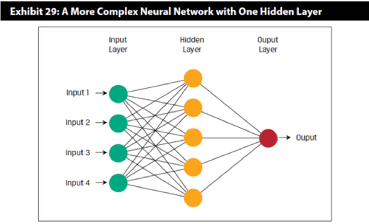
Neural networks have three types of layers:

an input layer (here with a node for each of the four features)

hidden layers, where learning occurs in training and inputs are processed on trained nets

an output layer (here consisting of a single node for the target variable y), which passes information outside the network.

At least 2, but often more than 20 hidden layers!!

The Reinforcement learning (RL) framework

involves an agent that is designed to perform actions that will maximize its rewards over time, taking into consideration the constraints of its environment.

Big data characteristics commonly referred to as the 3Vs

volume (quantity of the data),

variety (the array of available data sources),

and velocity (the speed at which data are created)

ML Model Building Steps

i) Conceptualization of the modeling task: determining what the output of the model should be

ii) Data collection

iii) Data preparation and wrangling

iv) Data exploration

v) Model training

Data cleansing is

the process of examining, identifying, and mitigating errors in raw data.

Data Wrangling (Preprocessing)

is performing transformations and critical processing steps on the cleansed data to make the data ready for ML model training.

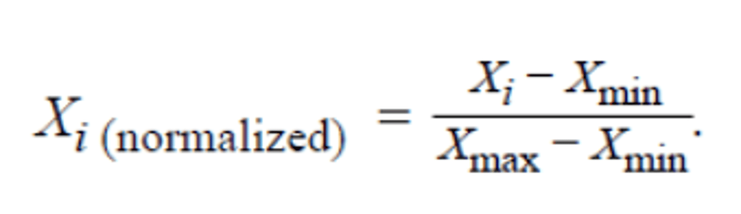
Scaling icin iki ana yöntemden Normalisation (Formula)

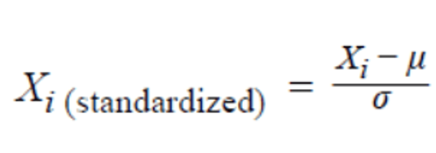
Scaling icin iki ana yöntemden Standartization (Formula)

Stemming

is the process of converting inflected forms of a word into its base word (known as stem).

For example, the stem of the words “analyzed” and “analyzing” is “analyz.”

Kelimeleri köküne indirgerken gramer veya anlam bilgisi dikkate alınmaz. Sonuçlar anlamsız olabilir ama benzer kelimeleri gruplayarak veri boyutunu azaltır

Lemmatization

is the process of converting inflected forms of a word into its morphological root (known as lemma).

For example, the lemma of the words “analyzed” and “analyzing” is “analyze.”

Daha doğru ama daha yavaş bir işlemdir.

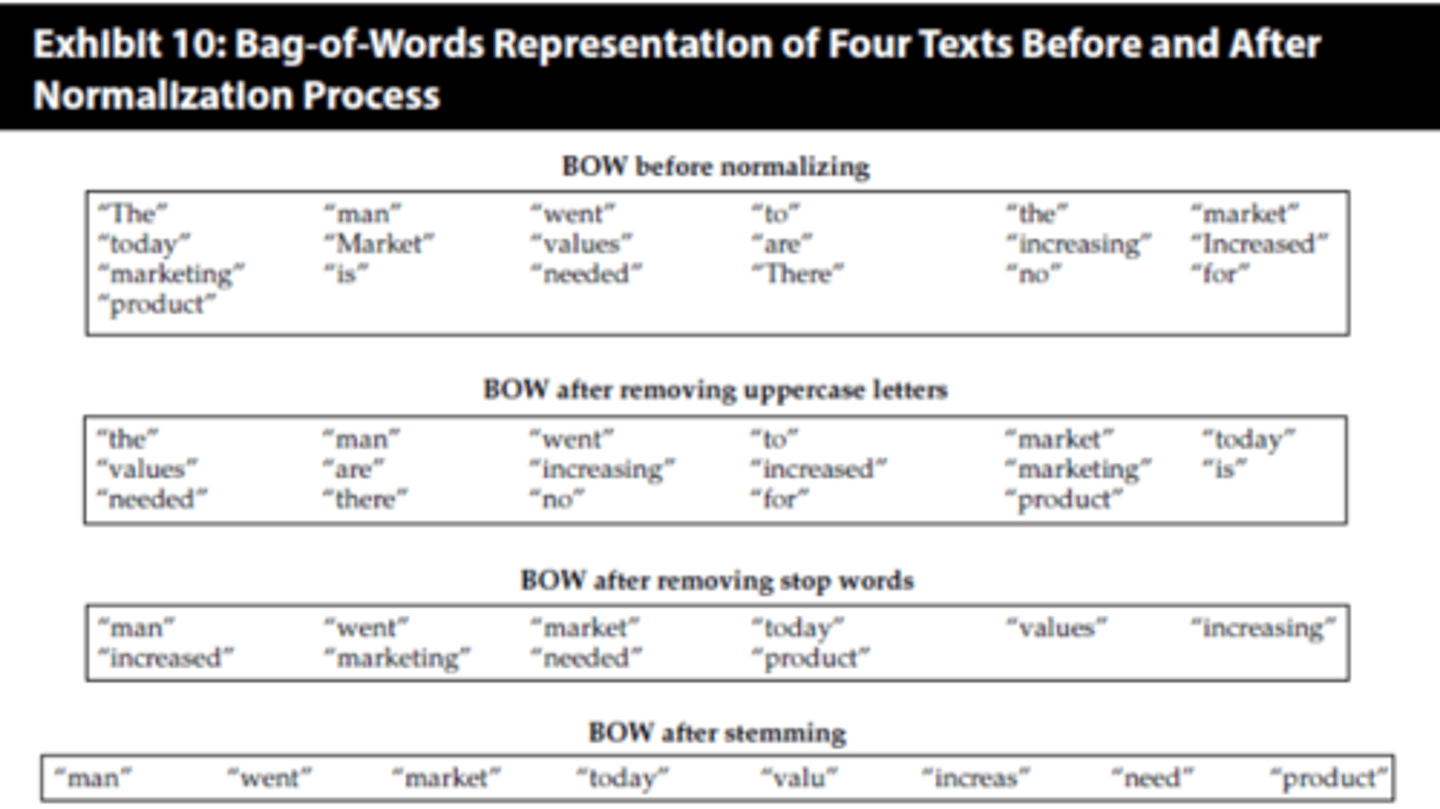
After the cleansed text is normalized, a XX is created.

a bag-of-words (BOW)

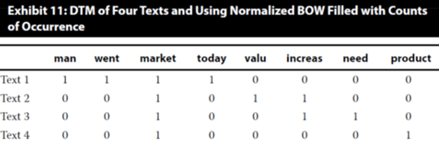
The last step of text preprocessing is using the final BOW after normalizing to build a XX.

Document term matrix (DTM)

Data Exploration Stage

N-grams

kelimeleri ardışık gruplar halinde ele alıp bağlamı yakalamamıza yarar.

Parts of speech (POS)

Tags each word with its grammatical role (noun, verb, adjective, proper noun, etc.) using language rules and dictionaries. (NER gibi ama dilbilgisel yonden analiz eder)

Bag-of-Words (BOW)

Metindeki her kelimeyi ayrı bir özellik (token) olarak sayar.

Kelime sırasını dikkate almaz, sadece hangi kelimelerin ve kaç kere geçtiğini önemser.

Hassasiyet (Precision - P) (formul)

TP= True positive FP= False positives (Type 1 Error)

Ne Zaman Kullanılır: Yanlış pozitiflerin maliyetinin yüksek olduğu durumlarda (yani, bir şeyi pozitif olarak yanlış etiketlemenin çok maliyetli olduğu durumlarda) hassasiyet önemlidir. Örneğin, pahalı bir ürünün kalite kontrolünde sağlamken hatalı olarak hurdaya çıkarılması gibi.

Duyarlılık/Geri Çağırma (Recall / Sensitivity - R) (formul)

TP= True positive FN= False positives (Type 2 Error)

◦ Ne Zaman Kullanılır: Yanlış negatiflerin maliyetinin yüksek olduğu durumlarda (yani, bir şeyi negatif olarak yanlış etiketlemenin çok maliyetli olduğu durumlarda) duyarlılık önemlidir. Örneğin, kusurlu bir pahalı ürünün kalite kontrolünden geçip müşteriye gönderilmesi gibi.

Doğruluk (Accuracy): (formul)

Doğru tahmin edilen sınıf sayısının (TP + TN), toplam tahmin sayısına (TP + FP + TN + FN) oranıdır.

F1 Skoru (F1 Score) (formul)

Hassasiyet (Precision) ve Duyarlılık (Recall) değerlerinin harmonik ortalamasıdır.

The more convex the ROC curve and the higher the AUC,

the better the model performance.

Öğrenmeye devam edilenler (5)

Bu terimleri öğrenmeye başladınız. Devam et!

Positive serial correlation in the residuals of a regression model typically results in

Type 1 errors

The number of dummy variables needed to distinguish among 4 different categories of companies is:

We need n − 1 dummy variables. So, if we use dummy variables to denote companies belonging to one of four categories, we use three dummies.

Here n = 4, so the number of dummy variables is n – 1 = 3.