BIOL 300 Midterm Memorize

conditions for binomial test 

• test whether a population proportion (p) matches a null expectation for the proportion 

• one variable 

• categorical variable 

• two categories (success, fail) 

what is the flow chart for deciding which test to use?

How many variables?

• ONE 

  • categorical 

    • 2 categories 

      • BINOMIAL TEST 

    • 2+ categories 

      • x² GOF - PROBABILITY DISTRIBUTION 

  • numerical 

    • x² GOF - POISSON DISTRIBUTION  

• TWO 

  • sample size assumption met 

    • x² CONTINGENCY TEST 

  • sample size assumption not met 

    • FISHER’S EXACT TEST 

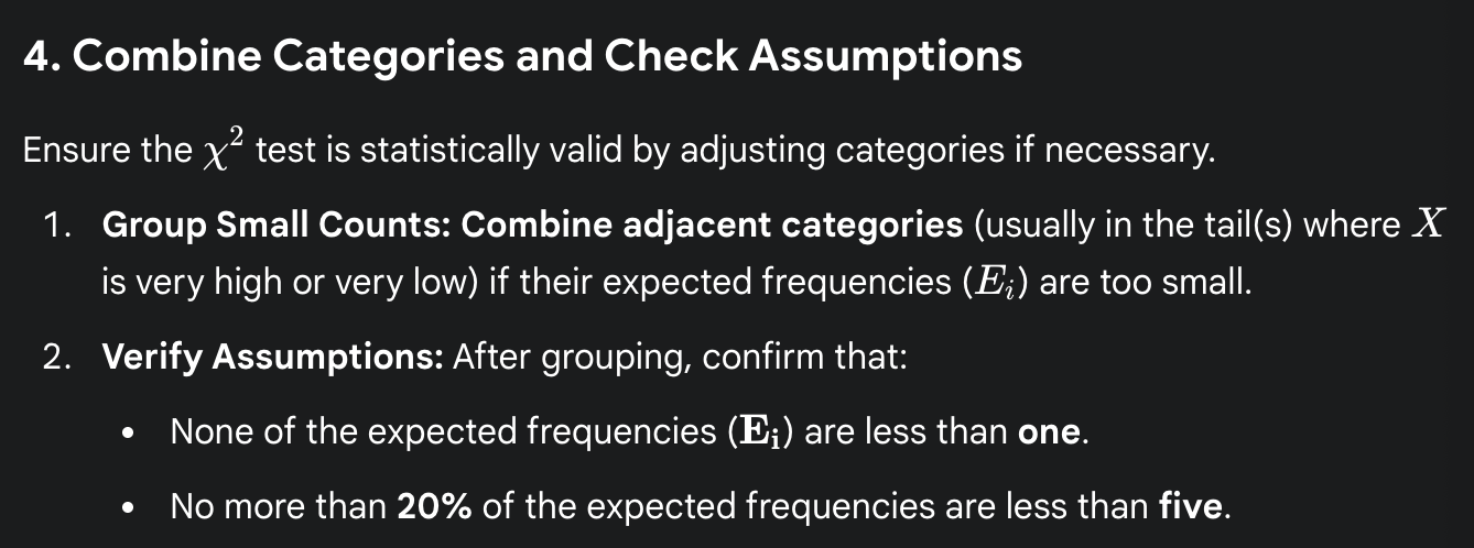
conditions for x² goodness of fit test

• use frequency data to test whether a population proportion equals a null hypothesized proportion that comes from a specified probability distribution

• use if sample size is too large for binomial test (can be very tedious to calculate the observed and more extreme many times; but less precise) 

• one variable 

• categorical or discrete numerical variable

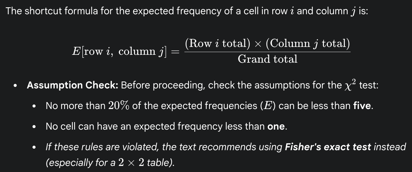
• no more than 20% of categories with expected < 5 & no category with expected < 1 & random sampling 

what are the conditions for the x² contingency test 

• want to test the association of two or more categorical variables

• two or more variables

• categorical variables

• no more than 20% of categories with expected < 5; no category with expected < 1; random sampling

what are the conditions for fisher’s exact test?

• want to test the association of two categorical variables by calculating the exact probability of the sample under the null hypothesis (useful when the assumptions of x² test are violated) 

• two variables 

• categorical variables 

• random sampling 

what are the test statistics for the binomial test, x² goodness of fit test, x² contingency test and the fisher’s exact test

(test statistic: value(s) calculated from the sample that are relevant to testing the null hypothesis)

binomial: p-hat (sample proportion) or x (number of successes of n trials)

• x is used to calculate p-hat

x² gof: x²

x² contingency test: x²

fisher’s exact test: none (not really done by hand)

how to decide over binomial test and x² gof test

• choose binomial when gof assumption not met 

• choose gof if too tedious to calculate probabilities of binomial (if gof assumptions are met as well) 

how to decide between x² contingency and fisher

• choose fisher if x² test assumptions are violated 

which tests have sample assumptions and what are they

• x² goodness of fit (probability distribution/poisson distribution)  & x² contingency

• no more than 20% of categories with expected values < 5; no category with expected < 1; random sampling 

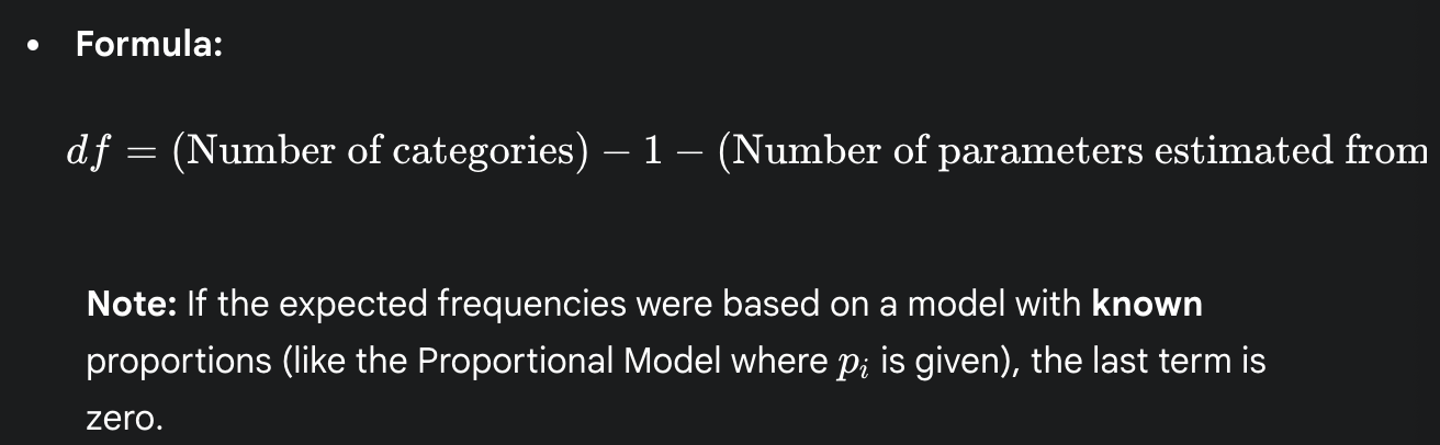
which tests use degrees of freedom and how do you calculate them?

x² goodness of fit test & x² contingency test 

gof: (# of categories) - (# parameters estimated from data) - 1

contingency: (# columns - 1) * (# rows - 1)

what are the null hypotheses for a binomial test, x² gof test, x² contingency test, and a fisher’s exact test?

binomial: the relative frequency of successes in the population is p0

(p = p0)

gof: the data come from a specified probability distribution (proportional, poisson, binomial)

contingency: the variables are independent 

fisher’s: the variables are independent

what are clear indicator to base a x² goodness of fit test on a poisson distribution and not some other distribution (proportional distribution)?

poisson 

• numerical discrete data

• being asked if events are randomly distributed in time or space 

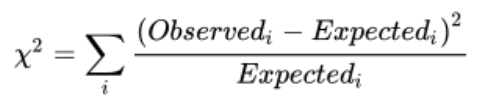
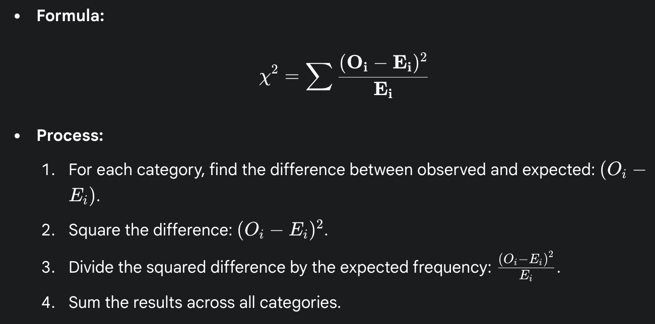
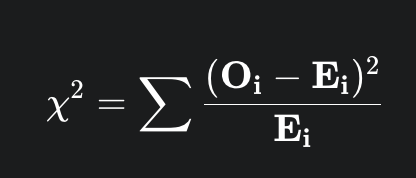
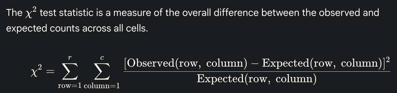
what is x² (chi-squared statistic)

• a single, non-negative number that quantifies the total discrepancy between a set of observed frequencies and the corresponding expected frequencies under a specific hypothesis

how does the use of x² compare and contrast in the goodness-of-fit test and the contingency test 

• same formula, differs in purpose and calculation of expected frequencies 

• gof: you are comparing your data to an external blueprint (the expected distribution) 

• contingency: you are comparing your data to an internal standard (what would be expected if the two variables were unrelated, as derived from the table’s own margins) 

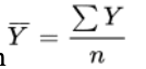
sample mean formula

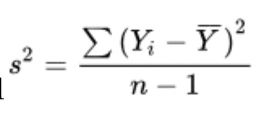
sample variance formula

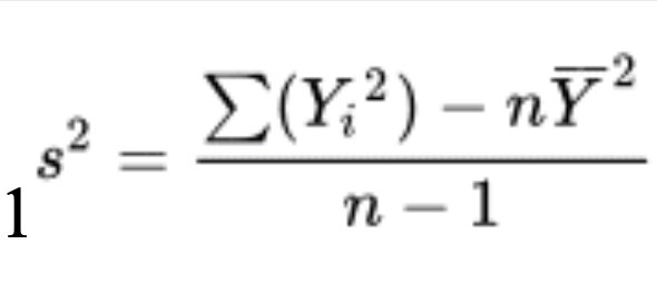
sample variance shortcut formula

sample standard deviation

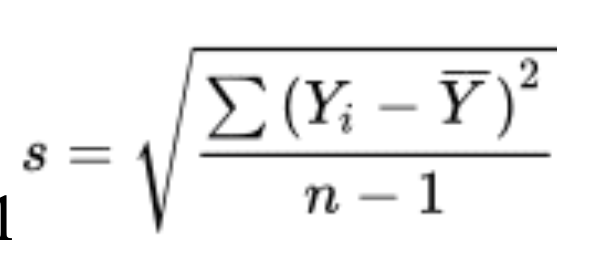
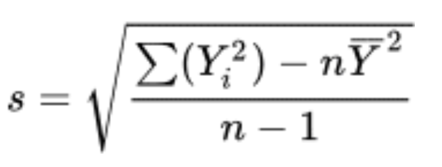
sample standard deviation short cut

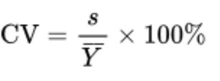
coefficient of variation formula

median

the middle observation (if the number of observations is even, average the middle two values)

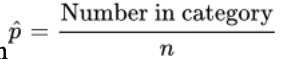
sample proportion + formula

how does adding a constant to all the measurements of a sample mean change it? 
how does multiplying all the measurements of a sample mean change it?

• the constant is added to the sample mean 

• the sample mean is multiplied by the constant 

how does adding a constant to all the measurements of a sample variance change it? 
how does multiplying all the measurements of a sample variance change it?

• adding a constant does not change the variance 

• for multiplication the variance is multiplied by the constant squared (s² * c²) 

how does adding a constant to all the measurements of a median change it? 
how does multiplying all the measurements of a median change it?

• the constant is added to the median 

• the median is multiplied by the median 

how does adding a constant to all the measurements of a IQR change it? 
how does multiplying all the measurements of a IQR change it?

• the IQR is the same when adding 

• the IQR is multiplied by the absolute of the constant (only positive) 

sample error of the mean + formula

measures the precision of the sample estimate (y-bar) of the population mean (mu) 

• assumes that the sample is random 

• we have to estimate this because we do not normally know the true standard deviation of Y in the population 

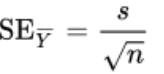
• s = sample standard deviation 

• n = sample size

parameter: 

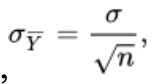
• but we do not know the standard deviation of the population 

Pr[A and B] for mutually exclusive events

0

Pr[A or B] for mutually exclusive events

Pr[A or B] = Pr[A] + Pr[B]

• addition rule 

Pr[A or B] for not mutually exclusive events

Pr[A or B] = Pr[A] + Pr[B] - [Pr A and B]

• general addition rule 

Pr[A and B] for independent events

Pr[A and B] = Pr[A]Pr[B] 

• multiplication rule 

Pr[A and B] for dependent events 

Pr[A and B] = Pr[A]Pr[B|A]

• general multiplication rule 

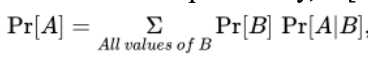
Law of total probability formula

binomial distribution probability formula

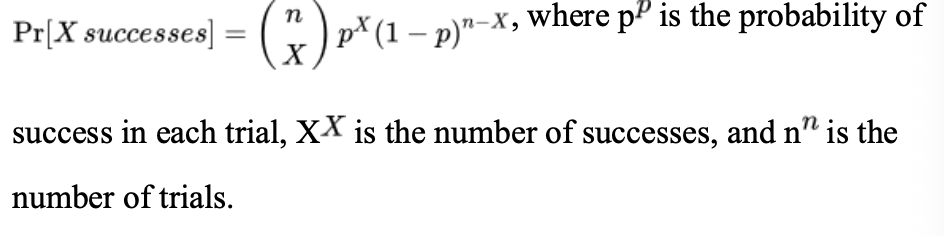
(n X) = n! / (x!(n-x)!)

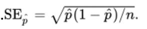
estimate of the standard error of a proportion formula

agresti-coull 95% confidence interval for a proportion 

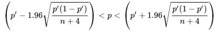
p’ = (X + 2)/(n + 4) 

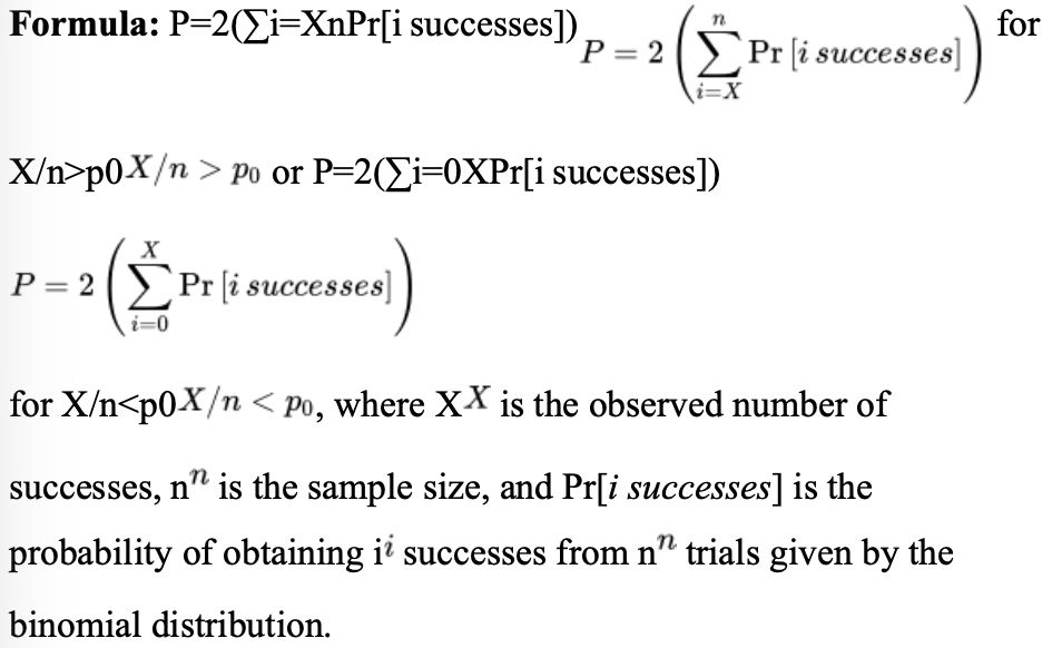
binomial test p-value formula

2*(sum of the observed probability and more extreme)

what can you do to meet the assumptions of x²

combine categories

when is the null hypothesis rejected for x²

if the observed x² statistic exceeds the critical value of the x² distribution corresponding to a 

what does comparing the variance of the number of successes per block of time or space to the mean number of successes do?

measures the direction of departure from randomness in time and space

• if the variance is greater than the mean, the successes are clumped

• if the variance is less than the mean, success are more evenly distributed than expected by the poisson distribution 

formula for the x² test statistic 

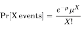
formula for the poisson distribution

(describes the number of independent events that occur per unit of time or space) 

odds of success + formula

probability of success divided by the probability of failure

the odds ratio

the odds of a focal outcome in one of two groups (treatment group) divided by the odds of that outcome in the second group (control)

• used to quantify the magnitude of associations between two categorical variables, each of which has two categories 

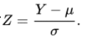
z-standardization + formula

converts values from any normal distribution with known mean and known standard deviation into standard normal deviates 

what are the steps to perform a binomial test? 

1. state null and alternative 

• H0: p = p0

2. determine the number of successes

• what will be used to compute a test statistic (proportion) that we will compare against the null expectation 

3. calculate p-value using the binomial formula 

• the probability of observing a result as extreme or more extreme than the observed statistic (X) assuming the null hypothesis is true

• use the binomial formula to calculate the probability of the observed and more extreme for one of the tails then multiply by 2 

4. draw conclusions 

• based on if p is larger or smaller than alpha (0.05 if not mentioned) 

what are the steps to perform a x² goodness of fit test based on a probability distribution

1. state null and alt 

• null: frequency distribution of the observed data matches a specific probability model or set of expected proportions 

2. calculate expected frequencies (E)

• use the rule or probability model stated in the null to determine the expected frequency for each category 

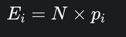
• the sum of all expected frequencies must equal the sum of all observed frequencies 

3. ensure that x² assumptions are true by checking expected frequencies 

• if assumptions are not met combine categories to increase the expected frequencies and then proceed with the new set of categories 

4. calculate the x² test statistic 

• x² measures the total discrepancy between the observed counts and the expected counts 

5. determine the degrees of freedom

• the df specify which x² theoretical distribution is used as the null distribution 

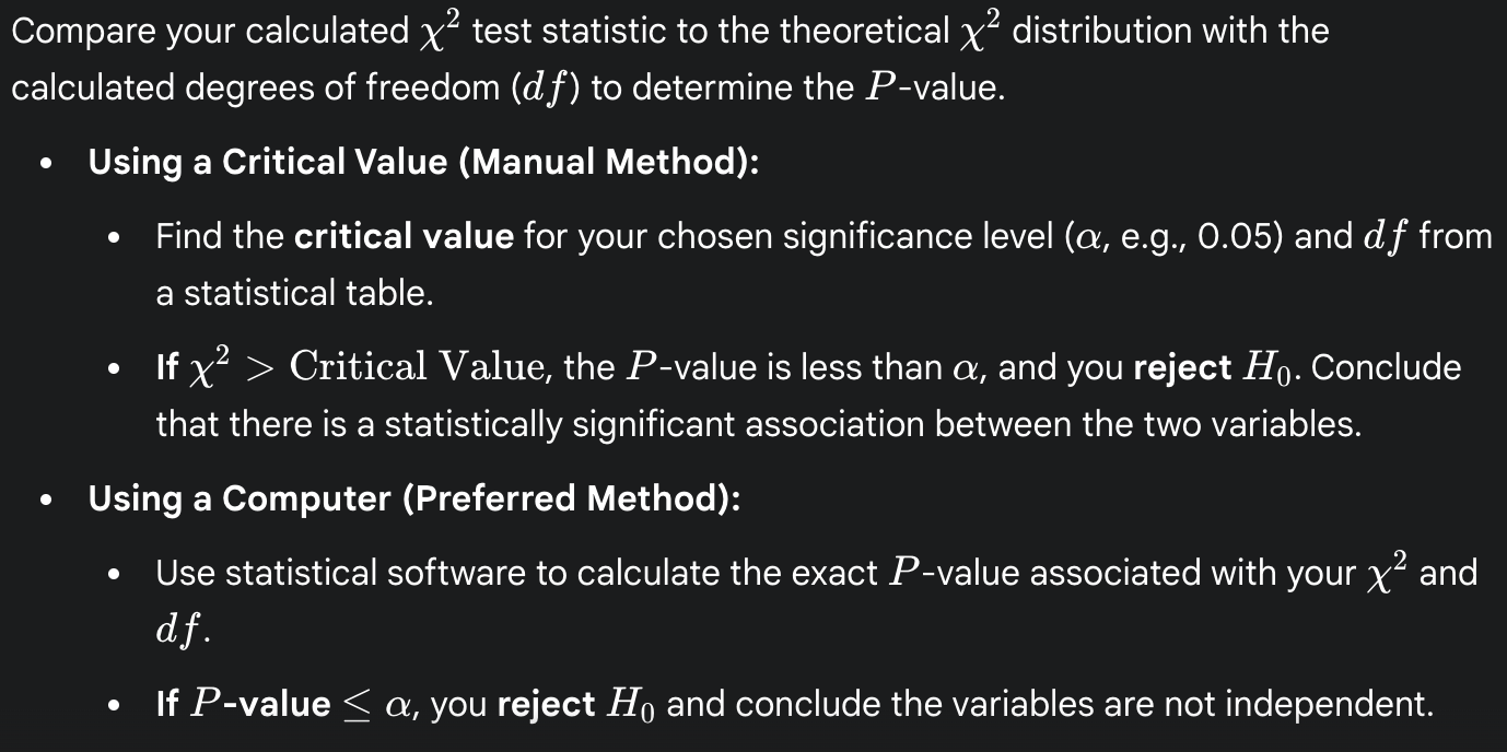
6. find the p-value and conclude

• compare the calculated x² statistic to the x² distribution with the calculated df 

• the p-value is the area in the right tail of the distribution

what is the critical value (in terms of x²)

the threshold on the x² distribution that separates the fail to reject and reject region 

1. choose the significance level 

2. look up the values in a x² critical values table 

• find the row corresponding to your df 

• find the column corresponding to a

• the intersection is the critical value

in an x² goodness of fit test (probability distribution) how does the critical value help us draw conclusions

since we only consider the right tail

• anything that is smaller than the critical value is considered more likely to happen

  • fail to reject the null 

  • p larger than alpha 

• anything that is larger than the critical value is considered less likely to happen 

  • reject the null 

  • p is smaller than alpha 

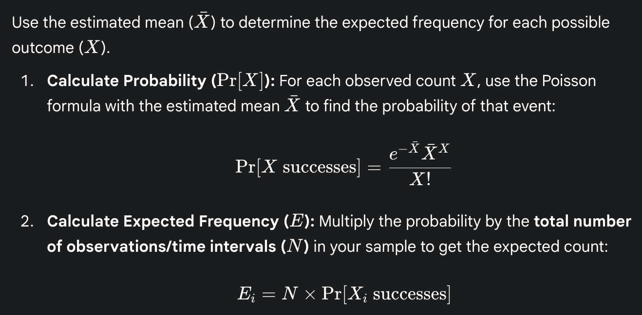
what are the steps to perform a x² goodness of fit test based on a poisson distribution?

1. state the null and alt 

• null: the number of successes per block of time or space has a poisson distribution 

2. estimate mean rate of the poisson distribution 

• since it is usually unknown, it must be estimated from your data 

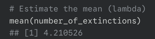
• calculate the sample mean of your observed count data. This value is used as the mu parameter in the poisson formula 

3. calculate the expected frequencies using the poisson formula

4. check assumptions and combine categories if needed

5. calculate the x² test statistic

6. determine the degrees of freedom

7. draw conclusions by comparing x² to the x² distribution with the determined df 

• if calculated x² statistic exceeds the critical value from the x² table, reject the null and conclude that the data does not follow a poisson distribution

what are the steps to perform a x² contingency test? 

1. state the null and alt

• null: the two categorical variables are independent

• alt: the two categorical variables are not independent 

2. organize the observed data

• arrange your sample data into a contingency table listing the observed frequencies for every combination of the two categorical variables 

• count the number of rows and number of columns in your table 

3. calculate the expected frequency for every cell in the table and check for assumptions 

4. calculate the x² test statistic

5. determine the degrees of freedom 

6. find the p-value and conclude 

how does a fisher’s exact test work and what are the steps to perform in computationally?

• an exact test unlike the x² contingency test which is an approximation 

• has no minimum data requirements 

• the test’s output allows you to determine if there is a statistically significant association (or lack of independence) between the two variables by providing a p-value 

• the R function also provides the odds ratio as a measure of the strength of the association 

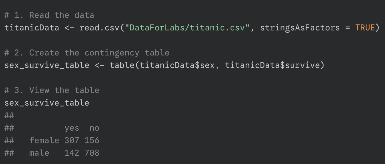
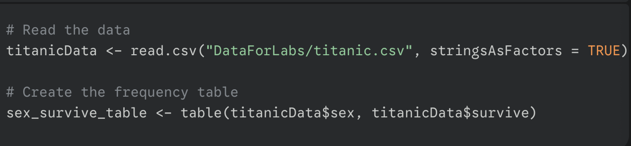
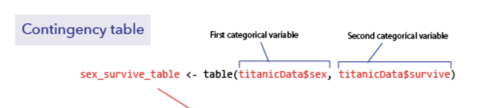
1. create a frequency table 

• test requires the data to be in a contingency table 

• after reading in data use table() command to create this object

• explanatory variable should come first 

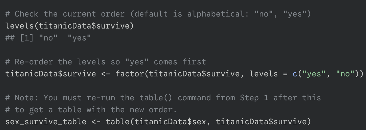
2. (optional) set the order of the factor level

• ensures the odds ratio is calculated with the probability of success in the numerator 

• default is alphabetical

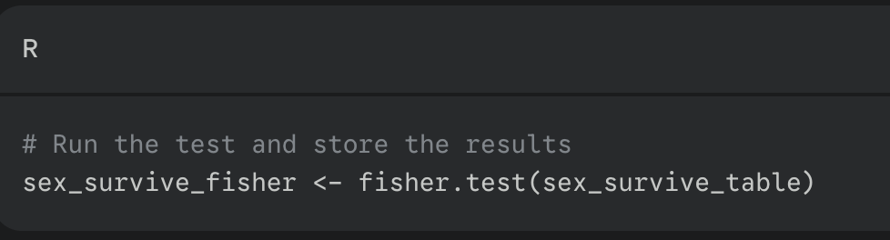
3. run the test 

• use the fisher.test() function providing your created frequency table as the input

3. interpret the results

• to get just odds ratio: sex_survive_fisher$estimate 

• to get just the 95 confidence interval: sex_survive_fisher$conf.int

what are the steps to perform a x² contingency test computationally?

1. create a frequency table using table()

• explanatory variable first

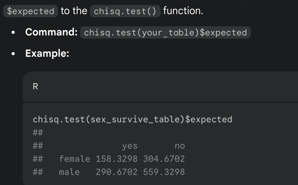
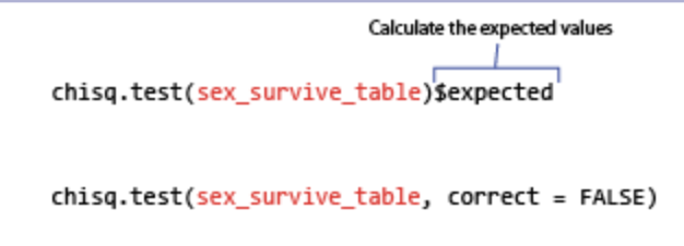
2. check the x² test assumptions (all expected values are greater than 1 and at least 80% are greater than 5) by using $expected 

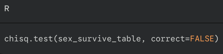
3. run the test using chisq.test() + correct = FALSE (to prevent a “Yate’s correction” which can be overly conservative)

4. interpret the results

• returns x² value, df and p-value

what is the function to run the fisher’s test?

fisher.test(table) 

what is the function to run the x² test 

chisq.test(table, correct = FALSE)

code: changing the position of categories

factor(data$column, levels = c(“name1”, “name2))

levels()

shows you the categories in a column and its order

what should you add when reading in data (esp for a fisher or contingency test) 

stringsAsFactors = TRUE

code: creating a mosaic plot 

mosaicplot(table)

• optional additions: colour = c(“colour1”, “colour2”), xlab = ““, ylab = ““

pulling odds ratio or confidence interval from a fisher test

object$estimate

object$conf.int

what are the steps to perform a x² goodness of fit test computationally? (probability and poisson)

• x² goodness of fit test compares observed category frequencies to the frequencies predicted by a null hypothesis

• either a null hypothesis specifies the probability or you estimate a parameter for your data (poisson distribution)

Case 1: probabilities given

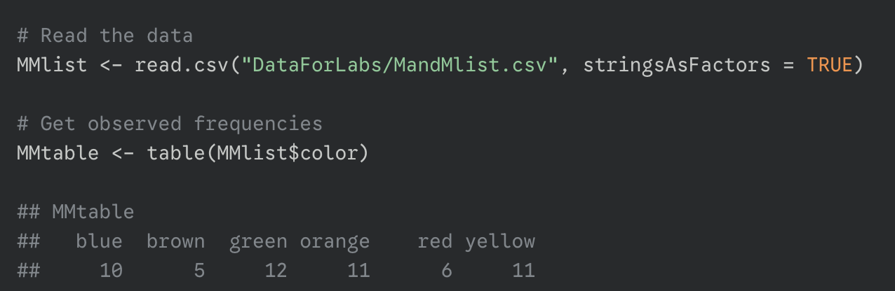
1. get observed frequencies using table()

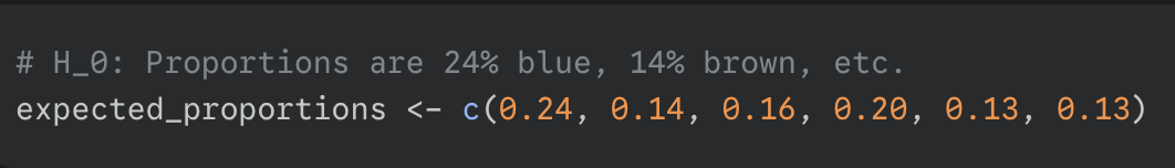
2. define expected proportions

• create a vector containing the expected proportions for each category as specified by your null hypothesis 

3. check the expected frequencies for test assumptions

• find the total sample size: sum(MMtable)

• calculate the expected frequencies: 55 * expected_proportions

• combine categories to meet expectations 

4. run the test by inputting expected_proportions to the chisq.test()

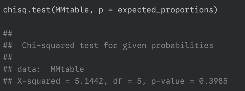
5. interpret results 

Case 2: Test with estimated parameters (poisson) 

1. get the observed frequencies using table()

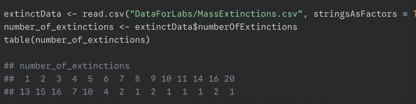
2. estimate parameters from the data

• the null hypothesis is that the data follows a poisson distribution, but the mean is unknown; so we must estimate it from the data 

3. calculate expected probabilities

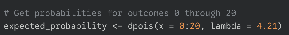
• using the estimated parameter use the dpois() function to find the expected probability for each possible outcome 

4. calculate the expected frequencies and combine categories 

• get the total sample size: length(column of interest)

• calculate expected frequencies by multiplying the probabilities by the total sample size: # * expected_probability

• check assumptions and combine

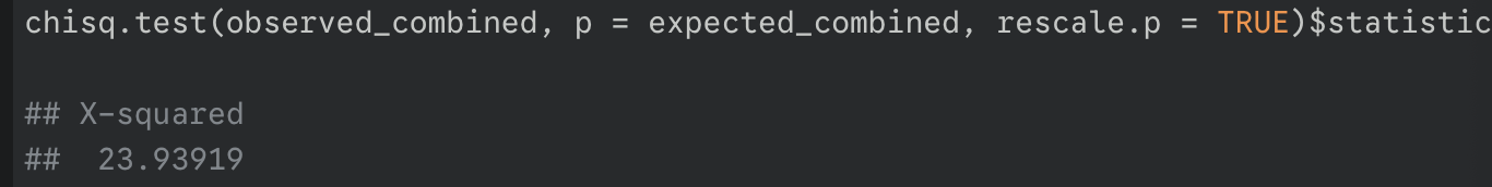
• create new vectors for your combined observed and expected frequencies

5. calculate the x² statistic using chisq.test()  and rescale.p = TRUE and $statistic

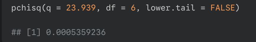
6. calculate degrees of freedom manually

• # of categories - 1 - # of estimated parameters

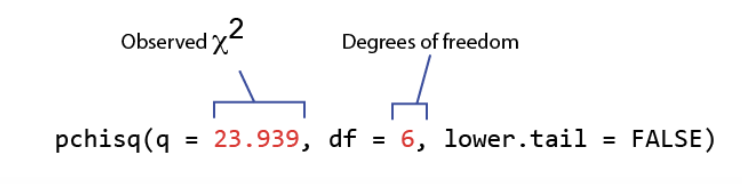
7. find the correct p-value using pchisq()

• give it your x² statistic (q) and your manually calculated df and lower.tail = FALSE to get the p-value (the area in the right tail)

8. interpret the result

dpois()

dpois(x, lambda)

• calculates the probability of getting x successes for a poisson distribution with a mean of lambda

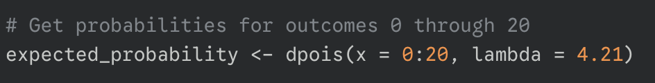
• calculates the probability of 0, 1, 2, … 20 successes given the estimate mean.

sum() vs length()

sum() 

• looks at the values inside a vector and adds them all together 

• can help you get sample size 

eg.

• sum(table(countries$continent))

  • table() creates the frequency table of counts

  • sum() adds those counts to get the sample size

length() 

• looks at the items in a vector and tells you how many there are 

• helps you determine how many categories 

eg.

• length(countries$continent)

  • length() counts the number of elements in the vector

how does running a x² test differ between no poisson and poisson?

probability distribution (no estimated parameter): 

chisq.test(x = tablewithexpectedfrequencies, p = exp_proportions)

poisson distribution (estimated parameter): 

chisq.test(x = obs_frequencies, p = exp_frequencies, rescale.p = TRUE)$statistic

followed by 

pchisq(q = x²value, df = manuallydetermineddf, lower.tail = FALSE)

what are the steps to perform a binomial test computationally?

1. identify the 3 required inputs of binom.test()

• x: the number of observed successes

• n: the total number of data points or trials

• p: the proportion specified by your null hypothesis

2. run the binom.test()

3. interpret the results based on p-value

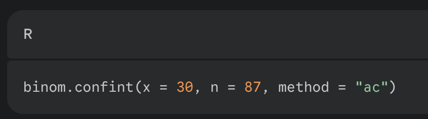
what are the steps to create a confidence interval for a proportion computationally 

1. load the binom package (to use the Agresti-coull method) 

• library(binom) 

2. run the binom.conf() function with method = “ac”

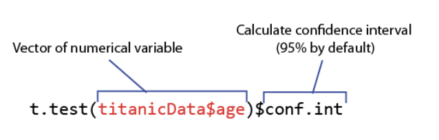
code: confidence interval of mean

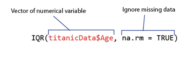
code: interquartile range

code: coefficient of variation 

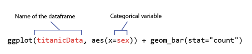
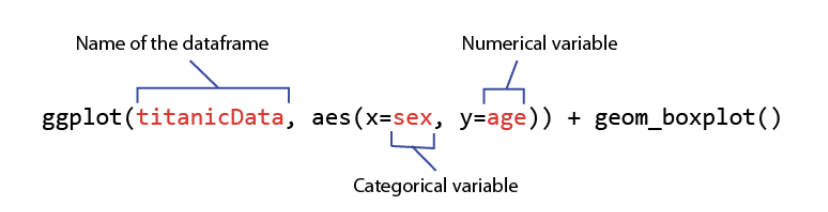
code: bar graph

code: boxplot

code: x² contingency analysis 

code: p-value from x² statistic