AP Micro - Unit 3

inputs v outputs

inputs - 4 factors of production, what is needed

outputs - what we are producing

short run

• fixed plant size (land, factory, etc.)

• variable usage

• variable output

long run

• variable plant size (more land, more factories, etc.)

• entry and exit (new companies can come, go)

letters

• T = total

• A = average

• M = marginal

• P = product (means price when alone)

• C = cost

• F = fixed (does not change as output changes, taxes, fees, etc.)

• V = variable (wages, utility costs, etc.)

• MP = change in TP / change in input

• AP = TP / number of inputs

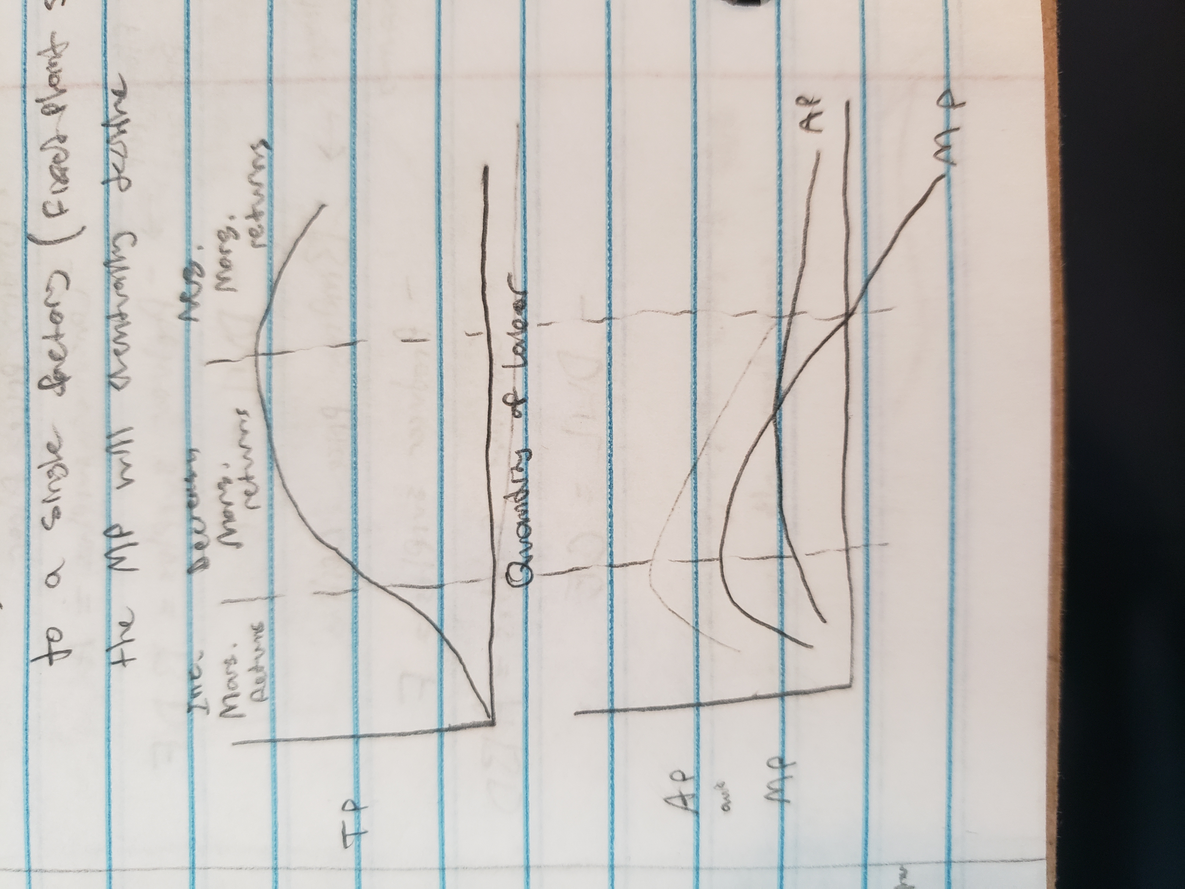
Law of Diminishing Marginal Returns

• As more of a variable resource is added to a fixed resource, at some point, the MP of the variable resource will decline

• ex, as we add more workers to a single factory (fixed plant), the MP will eventually decline

Fixed costs

• TFC

• average fixed costs = TFC / Q

Variable costs

• TVC

• AVC = TVC / Q

Total cost

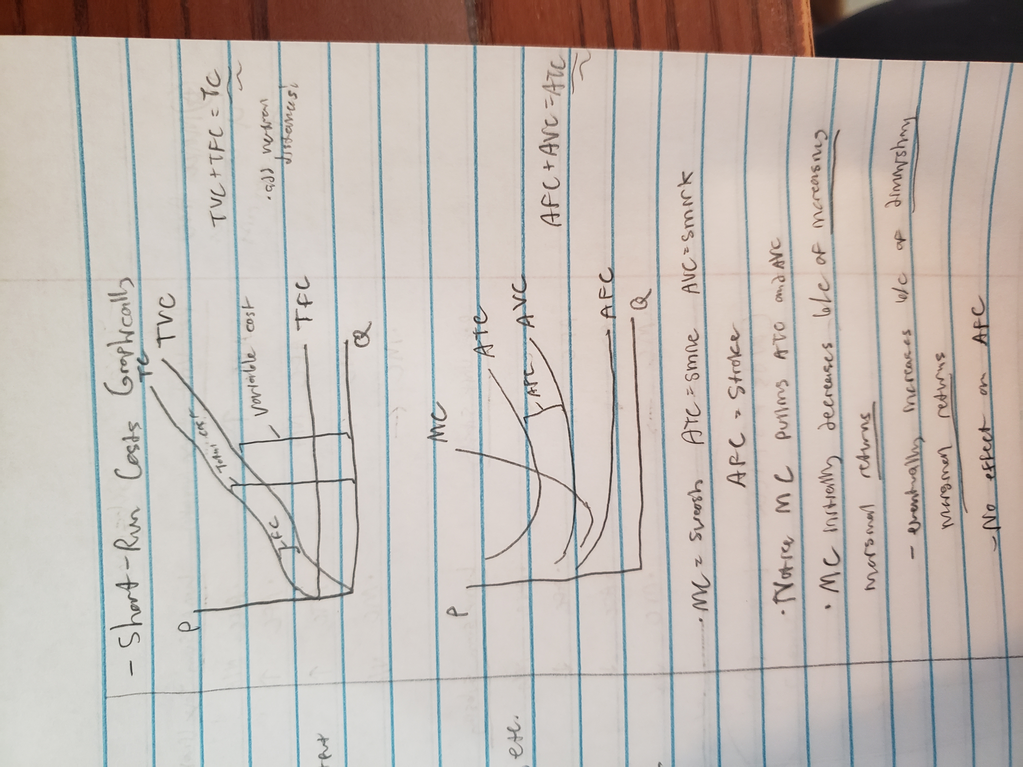
• TC = TFC + TVC

• ATC = TC / Q

marginal cost (MC)

• MC = change in TC / change in Q or change in TVC / change in Q

• fixed costs do not affect MC

effect of MP on AP

• if MP < AP, AP decreases

• if MP > AP, AP increases

• MC also controls AVC and ATC the same way

short run costs graphically

determinants of cost curves

• Productivity

  • Specialization

  • Division of Labor

  • Tech

• Input Prices

• Taxes / Subsidies

Shifting Cost Curves

• Higher costs will increase AVC and MC shifts left

• MC curves = supply curves for a company (which is why they shift left and right like one)

effect of per unit tax on AVC, AFC, ATC, MC

• AVC increases

• AFC (n/a)

• ATC increases

• MC shifts left

effect of per unit subsidy on AVC, AFC, ATC, MC

• AVC decrease

• AFC (n/a)

• ATC decrease

• MC shifts right

effect of lump sum tax on AVC, AFC, ATC, MC

• AVC (n/a)

• AFC increase

• ATC increase

• MC (n/a)

effect of lump sum subsidy on AVC, AFC, ATC, MC

• AVC (n/a)

• AFC decrease

• ATC decrease

• MC (n/a)

long-run production costs

• in the long run, all costs can change! No distinction between VC and FC

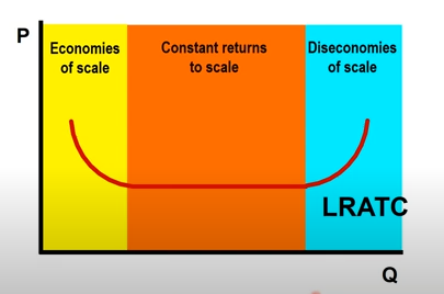
• P v. Q graph is a single, slightly U shaped LRATC curve (long run avg. total cost)

zones on a LRATC (and when will you see scale and return)

• econ of scale: growing businesses, efficient

  • Increasing output decreases LRATC

  • vs. increasing returns to scale, doubling input more than doubles output

• Constant returns to scale: doubling input doubles output

• diseconomies of scale: losing efficiency, doubling input less than doubles output

• “scale” = long run, “return” = short run

minimum efficient scale (MES)

• Lowest output where costs are minimized

• Larger output = industry more concentrated (fewer firms)

• on a graph, intersection between yellow and orange zones, or where it firsts hits minimum

explicit v. implicit costs

• explicit = monetary payments to others

• implicit = opportunity costs to owner, forgone salary, self-owned resources (PC, own car, own room)

  • forgone interest on static (one-time) payments / savings

accounting profit

• TR - explicit costs

economic profit

• TR - economic costs

• economic costs = explicit + implicit

• always smaller than accounting profit

normal profit

• implicit costs (what you could have had) (what you would have normally had)

short run profit maximization

• MR = MC rule

  • MR = extra revenue from selling one more unit = P (for now)

  • only works if you choose to produce

  • applies to all market models

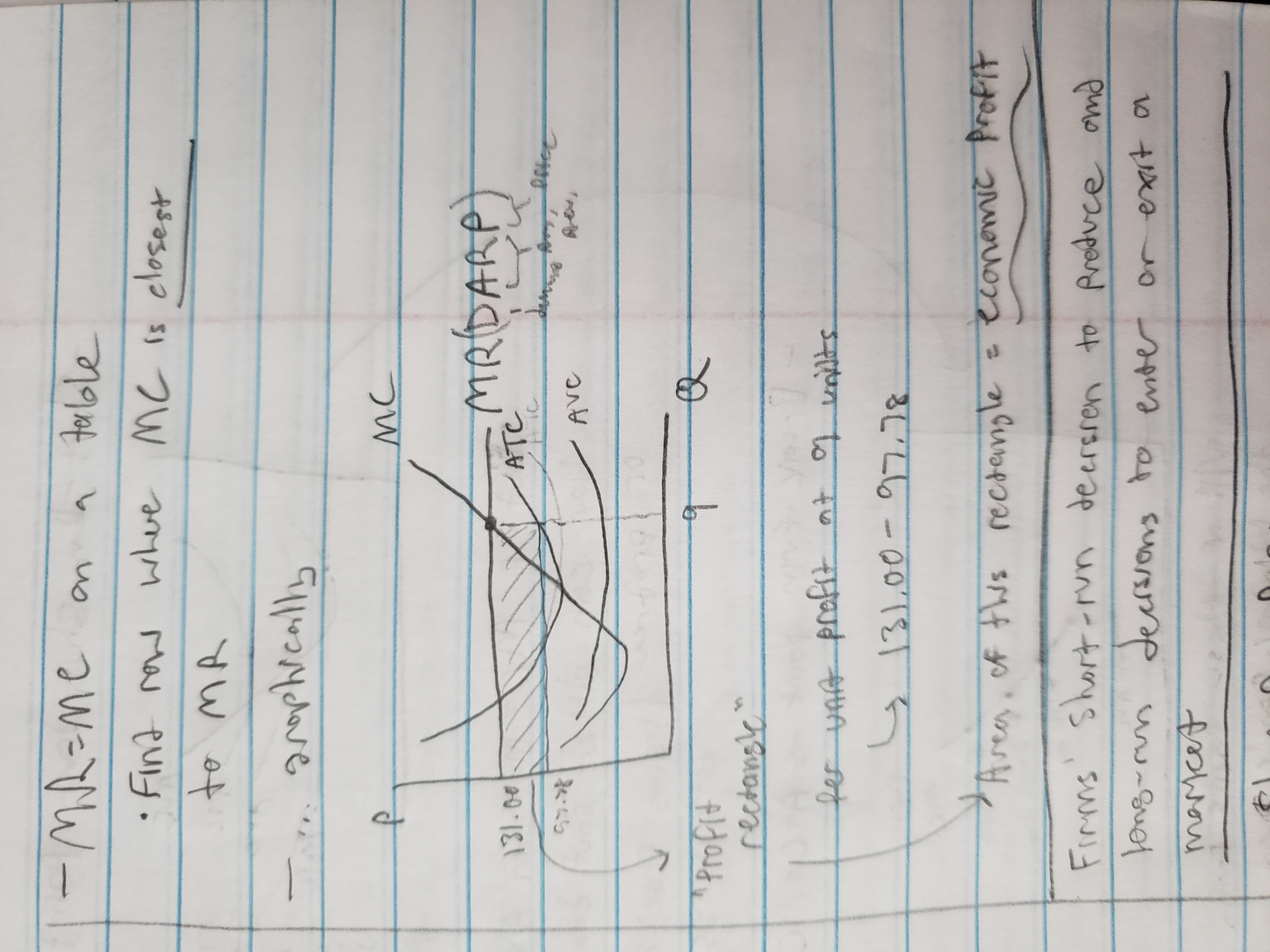
mr = mc rule on a table

• find row where MR is closest to MC, and/or where profit is the highest

mr = mc rule on a graph

MR = D = AR = P line

Study all images, know how to draw these graphs. Minimum of ATC and AVC should intersect with MC line

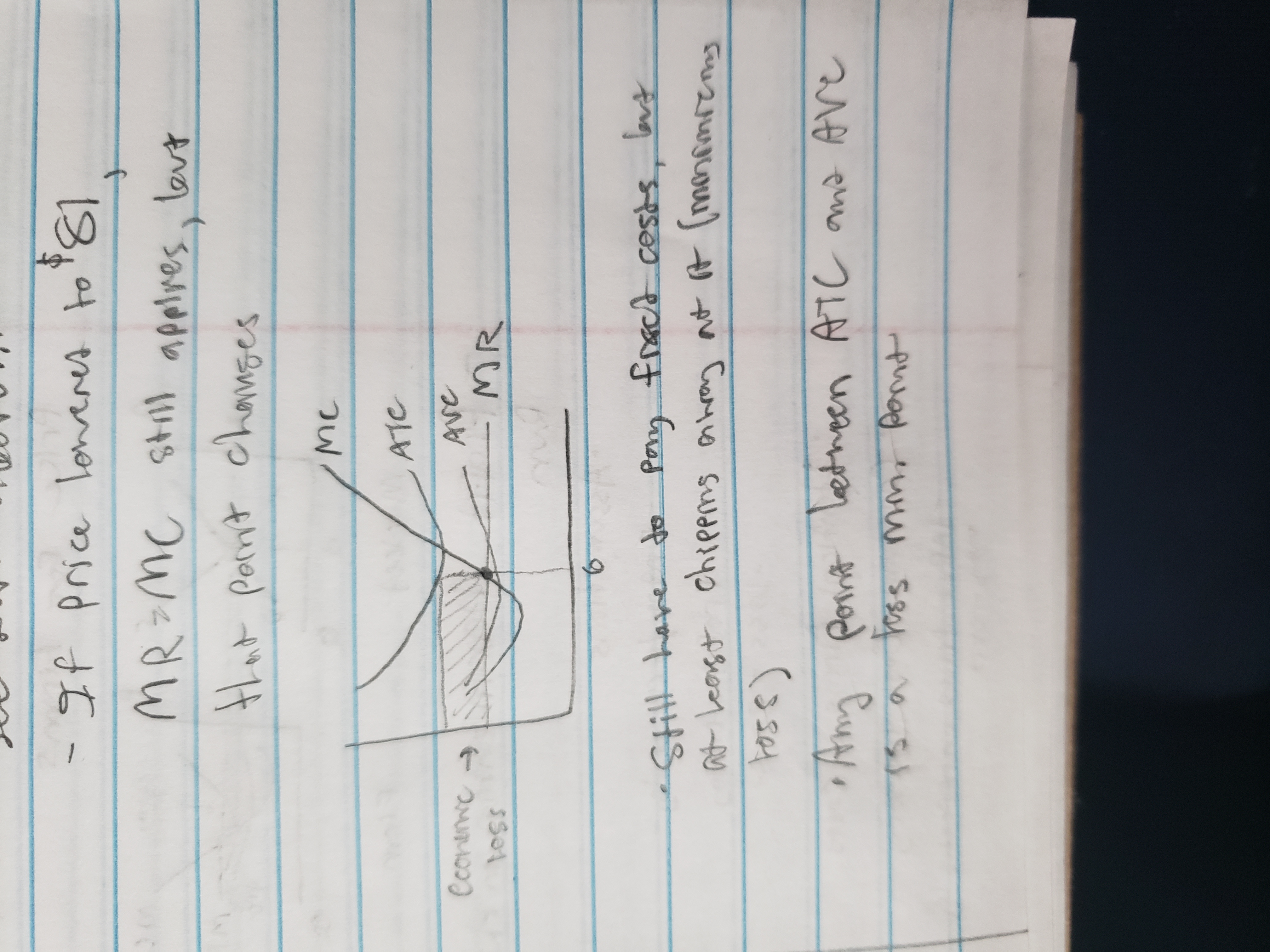
loss minimization position

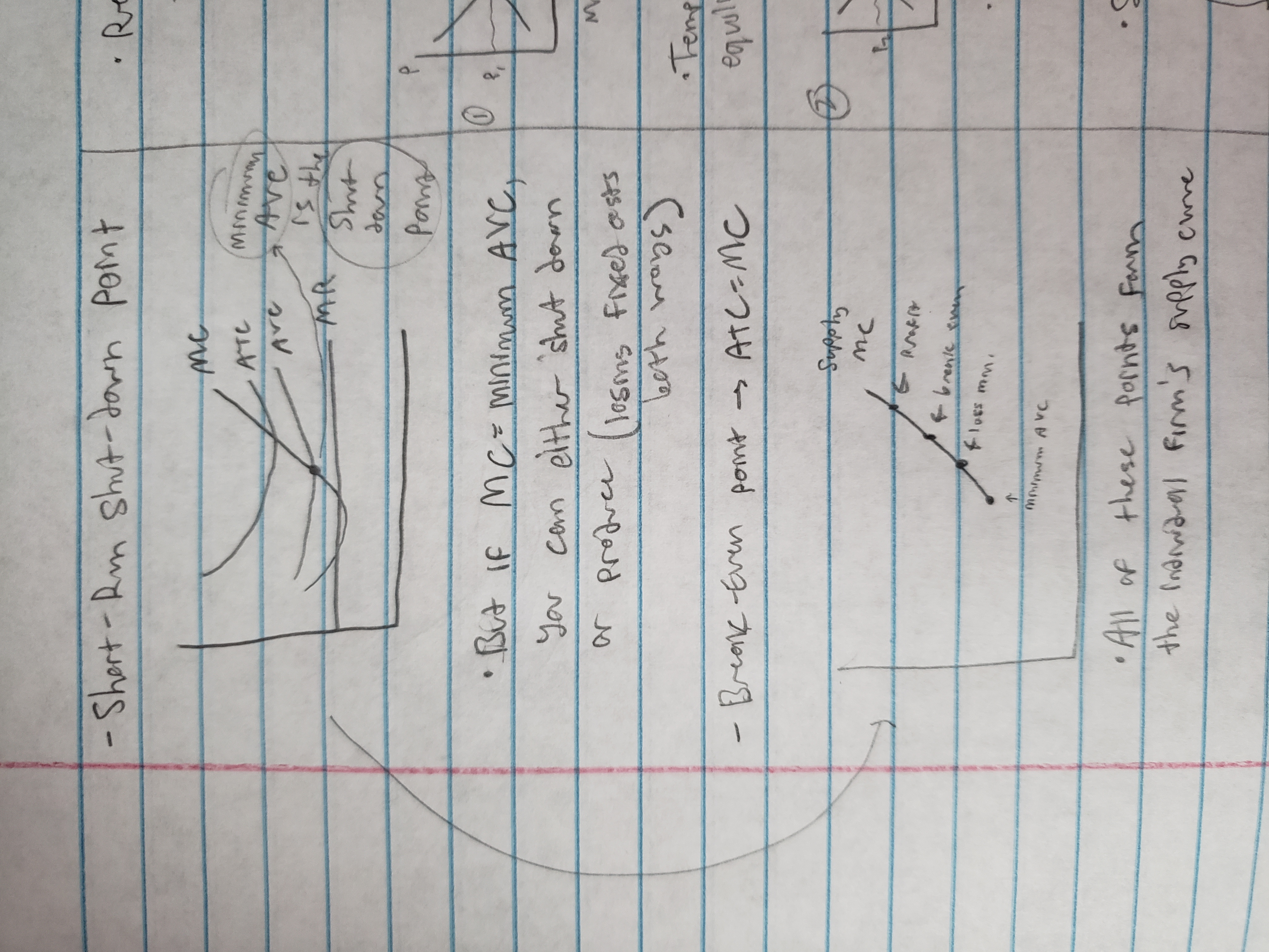
short run shut-down point and break-even point

side-by-side graphs (and why)

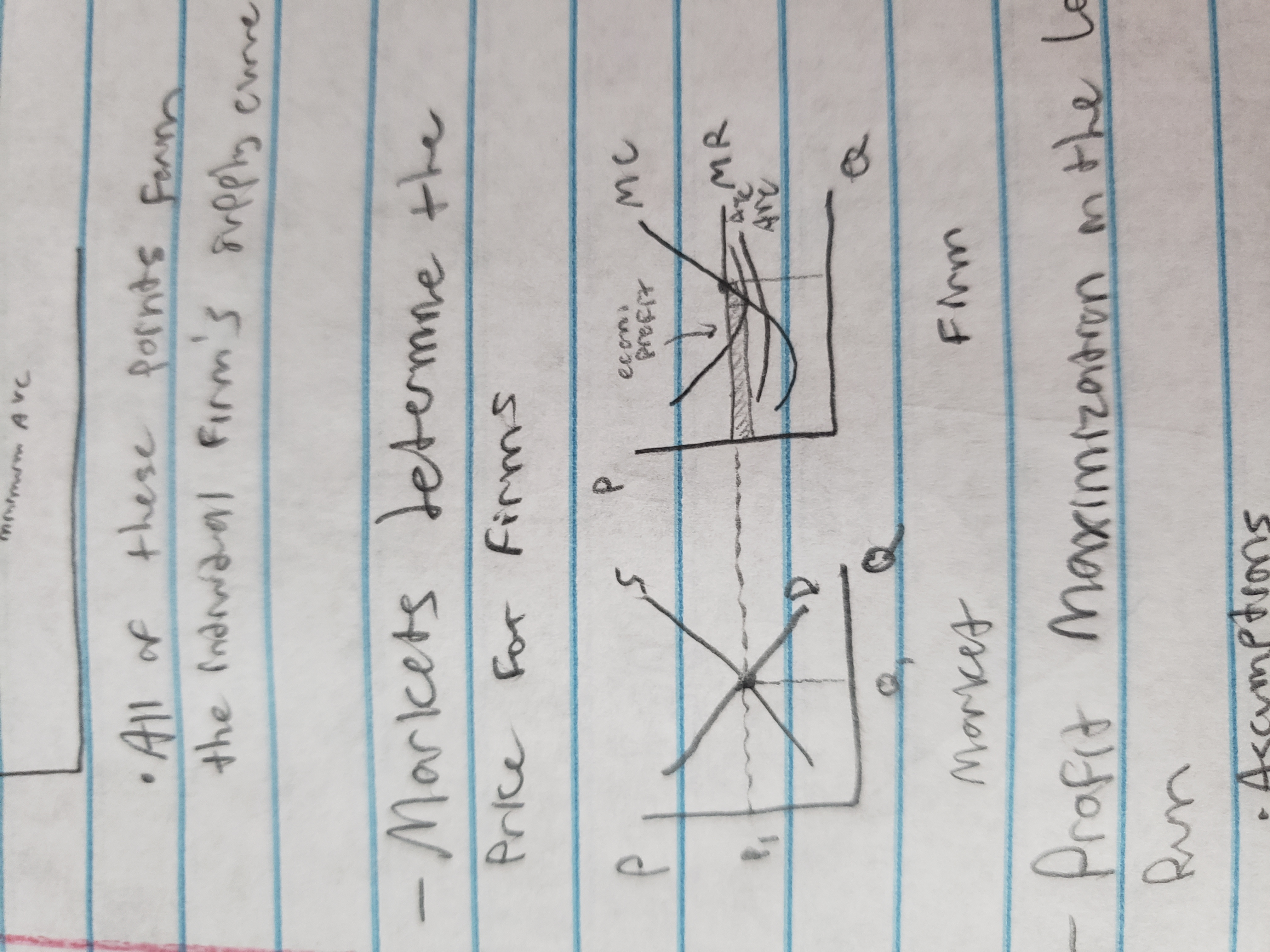
profit maximization in the long-run

• Assumptions

  • Entry/exit only (profit = entry, loss = exit)

  • Identical firms and costs

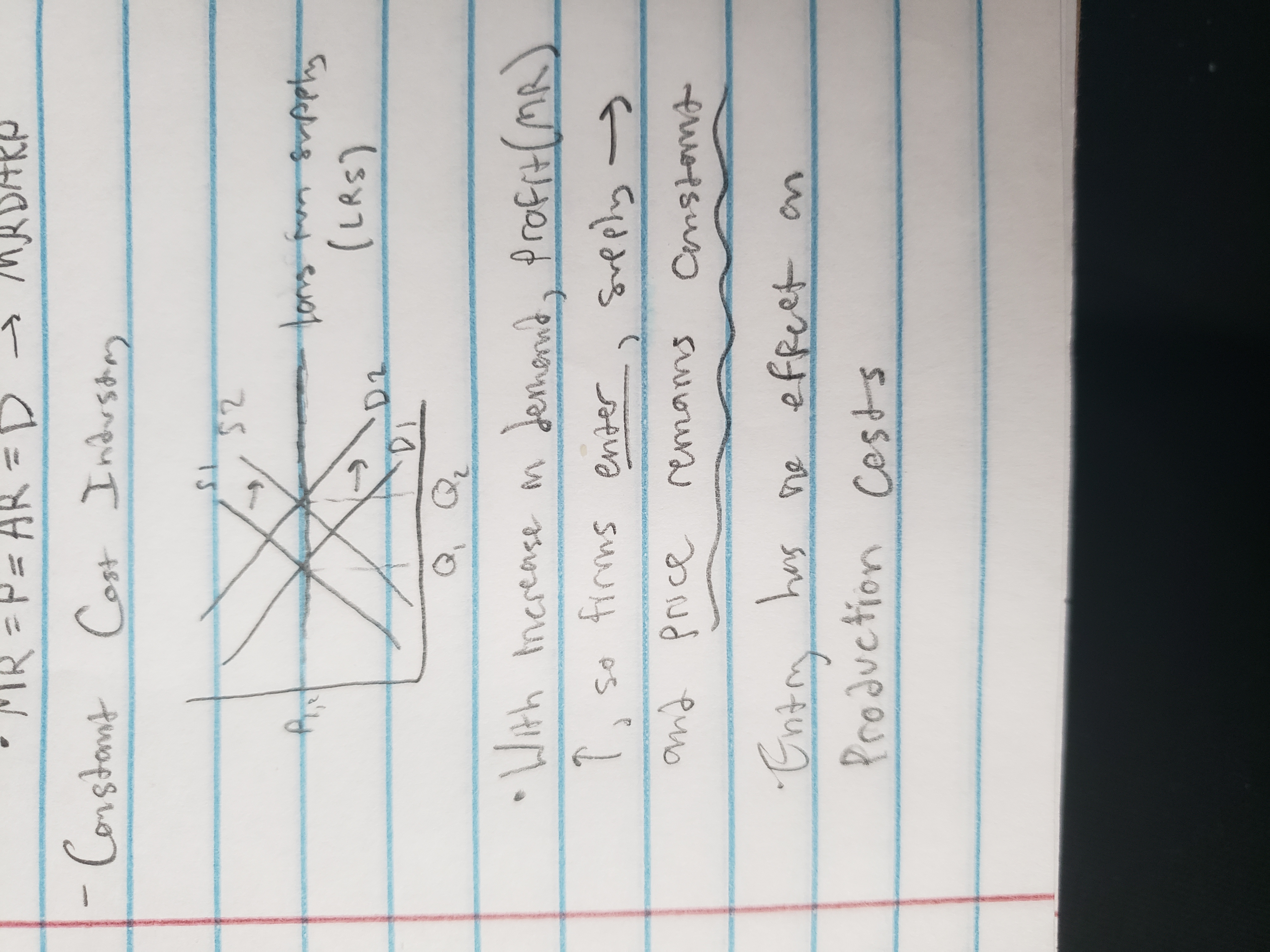
  • Constant-Cost industry (input prices unaffected by entry/exit)

• Results of analysis

  • MRDARP will end up at minimum ATC, and economic profit = 0

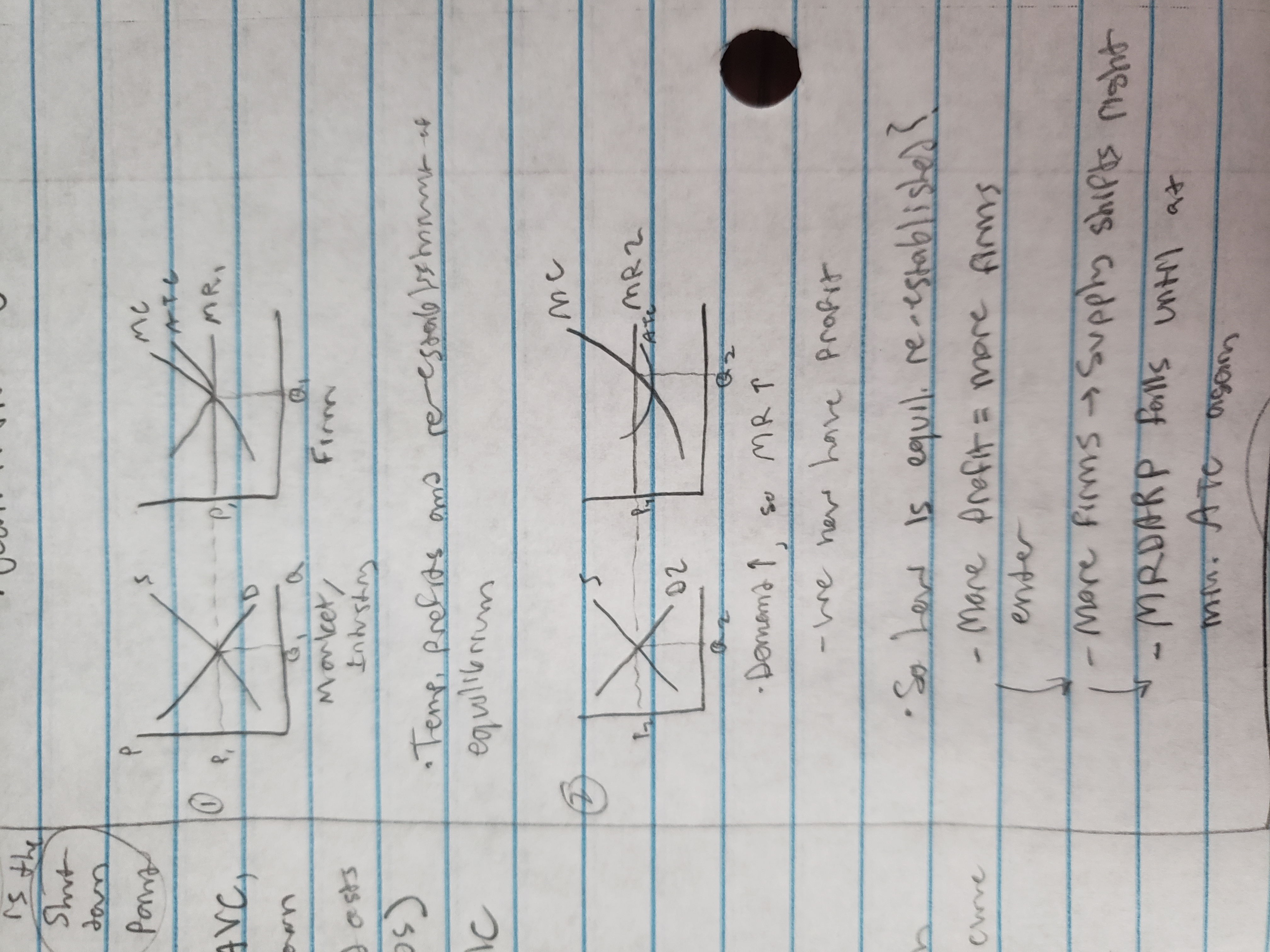
temporary profits, re-establishment of equilibrium (know thought process)

four market models (from most to least efficient)

• Perfect competition > monopolistic comp. > oligopoly > pure monopoly

perfect competition

constant-cost industry

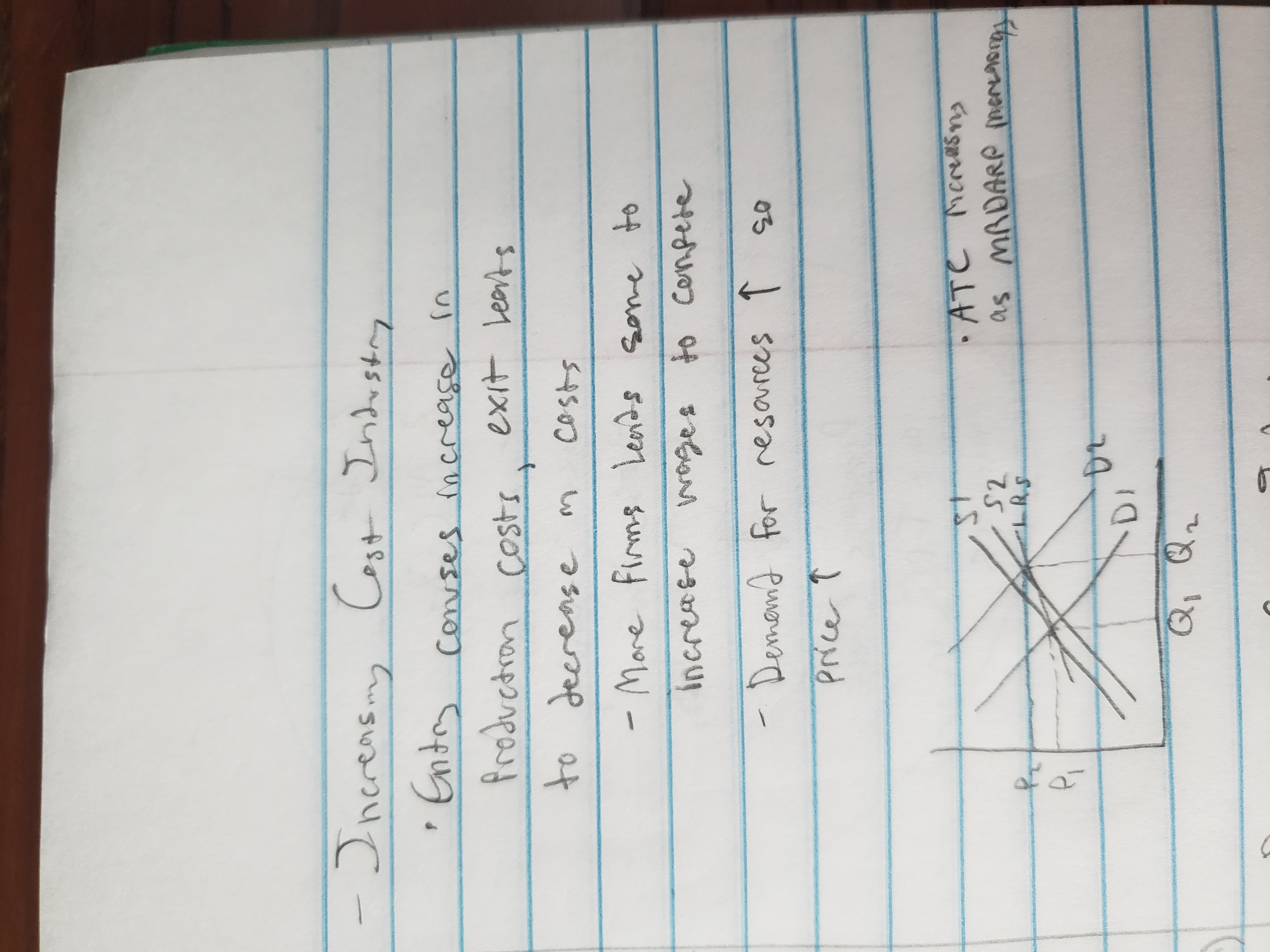
increasing cost industry

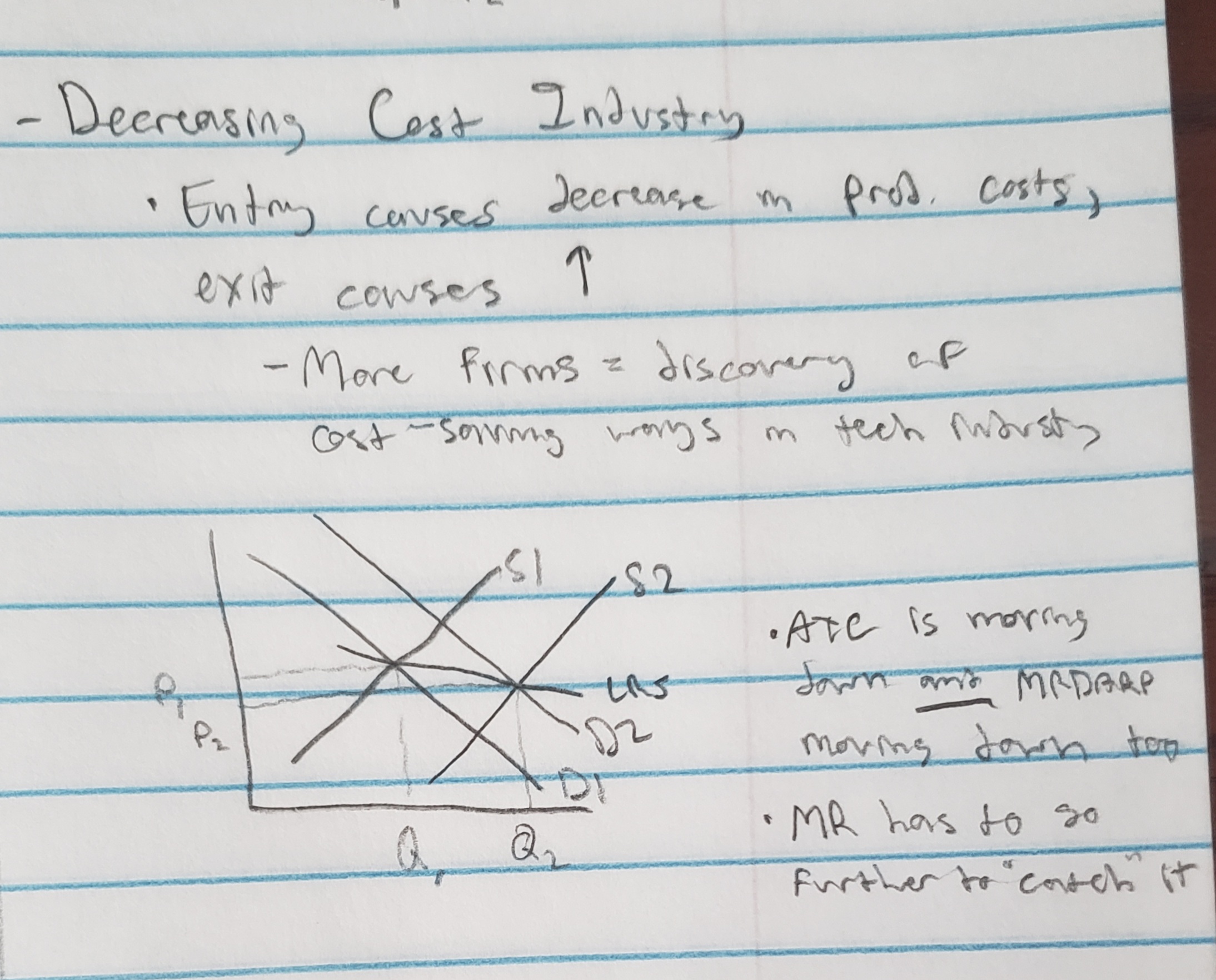
decreasing cost industry

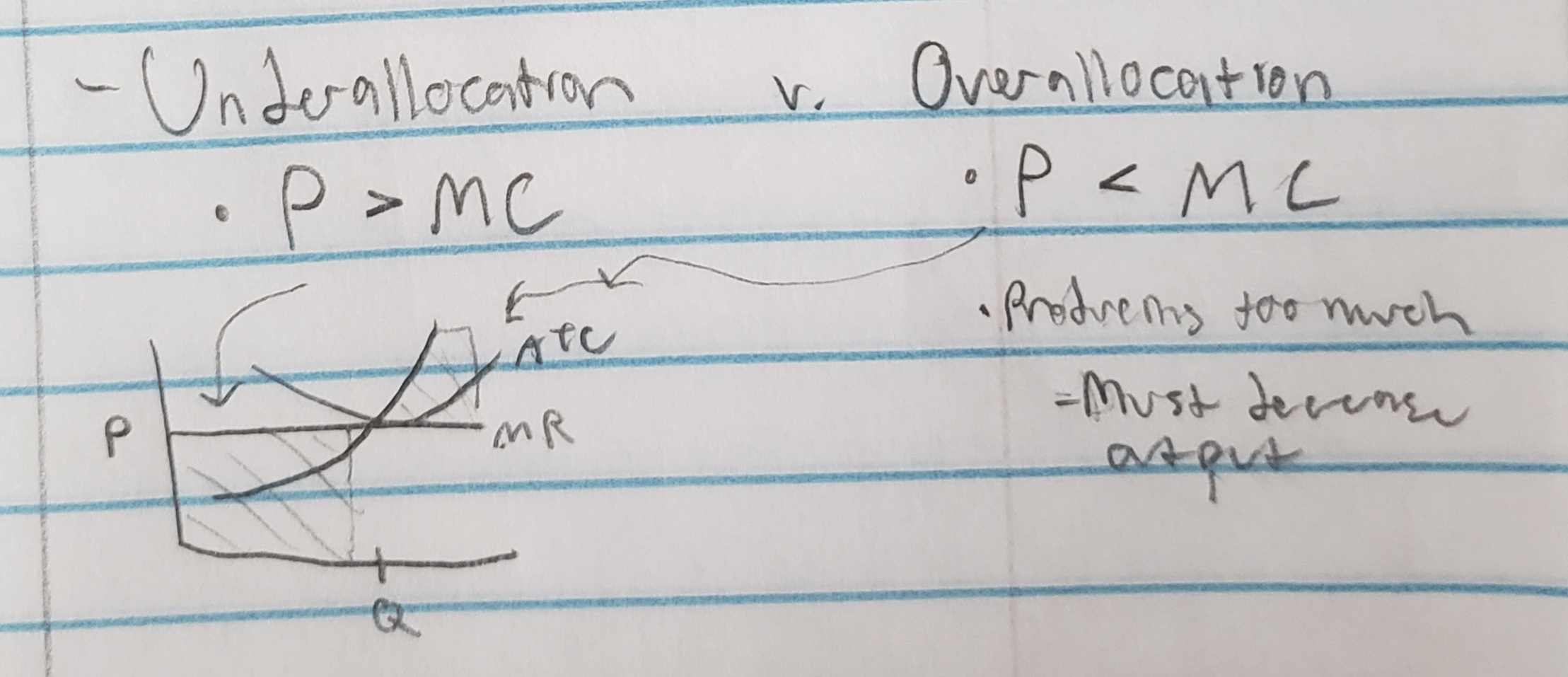
underallocation vs. overallocation, and what guarantees efficiency

• Perfect competition = productive efficiency (P = min atc, consumers getting product at lowest possible price) and allocative efficiency (P = MC, producing at the level society wants it to produce)