Test 2

Truncation Errors

Refer to errors in a method, which occur because some series (finite or infinite) is truncated to a fewer number of terms.

Such errors are essentially algorithmic errors and we can predict the extent of the error that will occur in the method.

(e.g. π ≠ 3.14 ≠ 3.14159 but they are approximate)

Round-off errors

Round off error occurs because of the computing device's inability to deal with inexact numbers.

Such numbers need to be rounded off to some near approximation which is dependent on the space allotted by the device to represent the number

Absolute Error

= true value - approximation

Shortcoming: an error of a micrometer is much more significant if we are measuring the size of a cell in comparison to the length of your arm.

So how do we account for the size of the error with respect to the magnitude of the measurement?

Fractional Relative Error

= (Absolute error/true value)*100%

The relative error gives an indication of how good the approximation is relative to the true value

These will be needed when we talk about propagating errors (i.e. combining multiple values that each have an error associated with it)

Variance

a measure of how data points differ from the mean

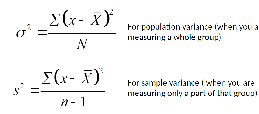
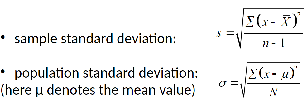
Standard Deviation

a measure of variation of scores about the mean

the average distance to the mean, although that's not numerically accurate, it's conceptually helpful. All ways of saying the same thing: higher standard deviation indicates higher spread, less consistency, and less clustering

Square root of variance

std() provides the sample standard deviation

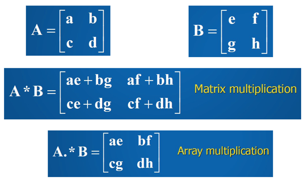
Dot-operations

use the “.” for element-by-element level

So use .* or ./ or .^ instead of * or / or ^

Matrix multiplication vs array multiplication

Use “.” before operator for array calculations

Defining Matrices

Enclosed in square bracket [ ]

Commas separate columns

Semicolons indicate a new row

Indexing arrays

Indexing can also be used to change values in a matrix or include additional values

Colon notation

Can be used to define evenly spaced vectors with a defined increment in the form:

first:increment:limit

linspace

Can be used to define evenly spaced vectors with a in the form

linspace(X1, X2, N)

generates N points between X1 and X2

Transpose

changes all of the rows of an array to columns and all of the columns to rows, B=A’

Concatenation

Creating a new matrix out of two previous matrices added as separate rows, C=[A; B]

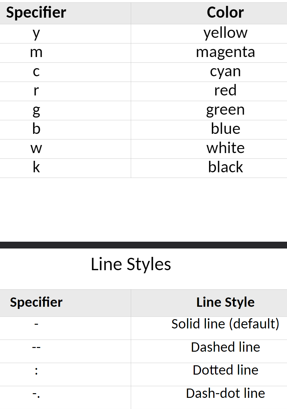
Plotting in 2D

1. Create 2 vectors

2. Use the plot(x,y,’format’) command

3. Will create a plot of y vs x

4. Format examples in pic

5. To plot again of same plot use the hold on command

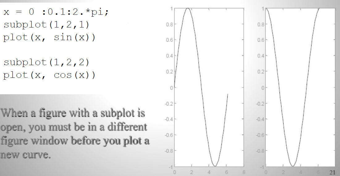
Subplots

Allows for putting multiple graphs in one figure

subplot(m,n,p) divides graphing window into a grid of m rows and n columns, where p identifies the part of the window where the plot will be drawn

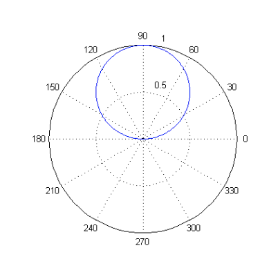
Polar plots

To plot polar coordinates (angle vs radius) use polar(angle,radius)

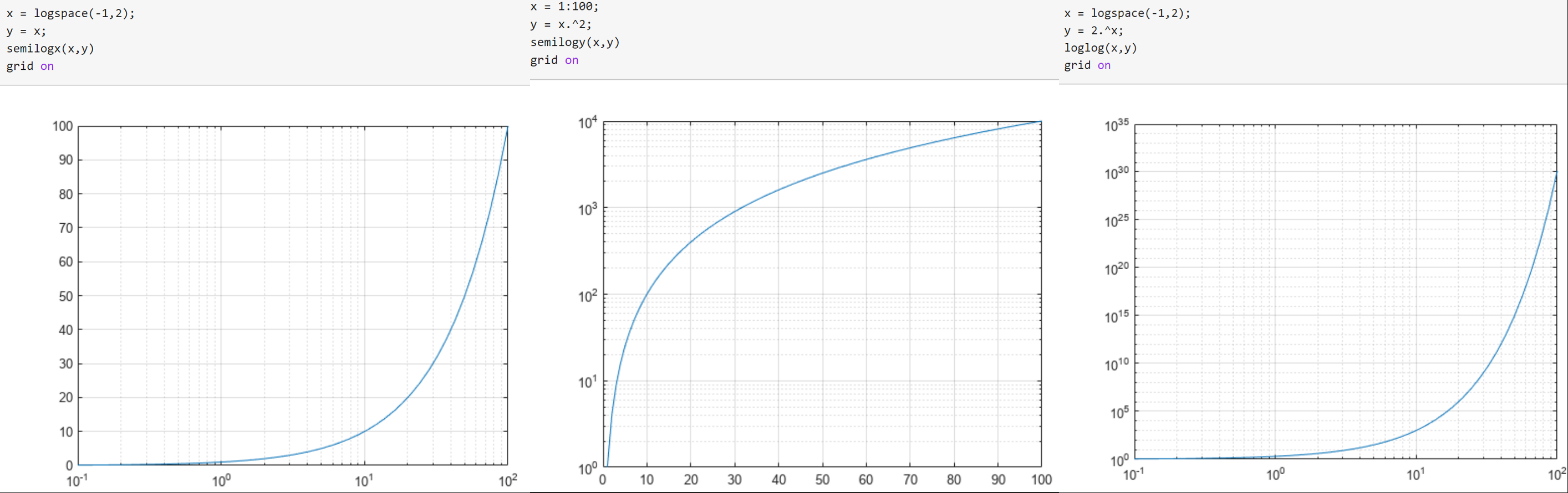
Logarithmic plots

3 kinds:

• semilogx

• semilogy

• loglog

Replace linear scales with logarithmic scales

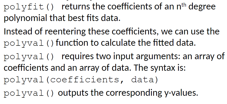
Linear regression

minimizes the squared distance between experimental data points and the modeled data points. This prevents positive and negative values from cancelling each other out

Use polyfit(x,y,polynomial degree) function with polyval() if necessary

fplot

“smart” command for plotting functions

Automatically analyzes the function to be plotted and decides number of plotting points to show all the features of the function

fplot(function,[xmin xmax])

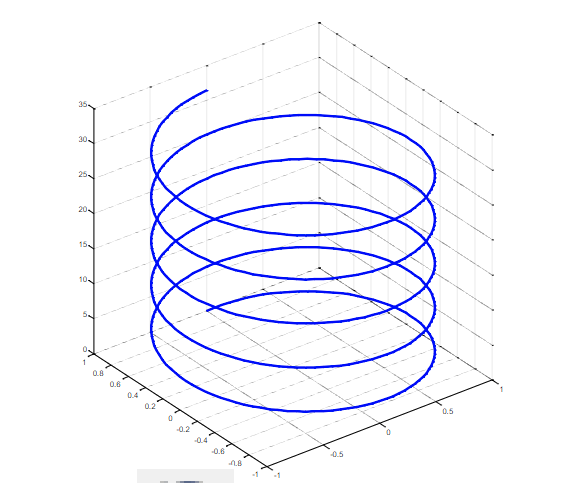
3D plots

plot3

graphs of 3 axes

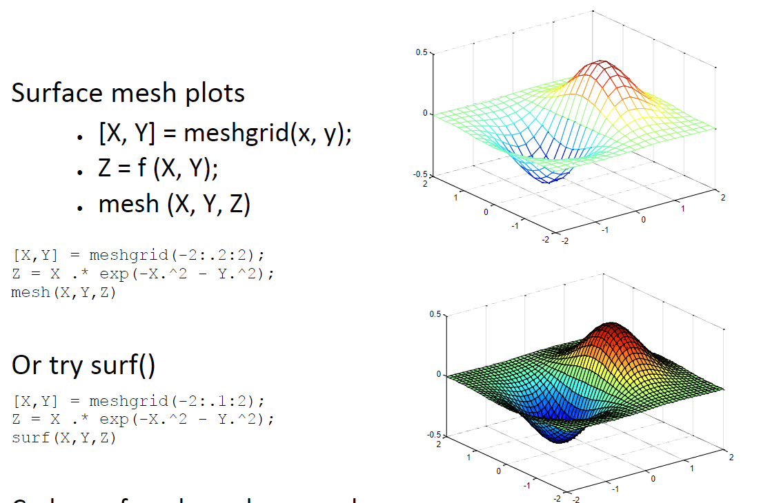
Surface mesh plots

meshgrid()

mesh(,,)

Create a rectangular grid out of an array of x values and an array of y values

To fill in the faces of the surface in color use

meshgrid()

surf(,,)

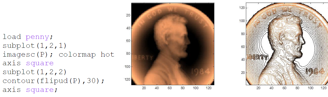
Contour Plots

a 3-D surface by plotting lines that connect points with common z-values along a slice

Things plots need

• a title

• axis label with the name of quantity and units

• same symbol of each data point in a given data set

• grid

• a legend

• regularly spaced tick marks at convenient intervals along each axis.

Syntax Errors

Syntax errors are errors in a MATLAB statement itself, such as spelling or punctuation errors

Run time Errors

• illegal operations

• exceeds the dimensions of that matrix

Logical Errors

• when the program runs without displaying an error, but produces an unexpected result

• very difficult to find.

  • compare simple test cases with known correct results to find where errors occur

Less than

<

Greater than

>

Equal to

==

Less than or equal to

<=

Greater than or equal to

>=

Not equal to

~=

Logical Operator

Produces logical result (1 or 0), and &, not ~, or |

And (logical operator)

&

is true when all of its operands are true

Not (logical operator)

~

is true when its operand is false

Or (logical operator)

|

is true when one or more of its operands are true

Hierarchy of Operations

1. Parentheses ()

2. Exponentiation (.^)

3. NOT operator (~)

4. Multiplication (.*) and division (./)

5. Addition (+) and subtraction (-)

6. Less than (<), less than or equal to (<=), greater than (>), greater than or equal to (>=), equal to (==), and not equal to (~=)

7. AND operator (&)

8. OR operator (|)

VPA Arithmetic

MuPAD, vpa(), variable precision

in between for time and accuracy

Alternatives:

• Rational MuPAD: more accurate, exact result, slowest

• Numeric MATLAB: less accurate, faster, floating point

is Functions

ischar() input is character array

isfinite() input is finite

isinf() input isinfinite

isletter() input is alphabetic letter

isnumeric() input is numeric array

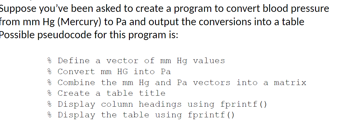
Pseudocode

Verbal description of your plan for writing a program

Written in English or as a combination of MATLAB code and English

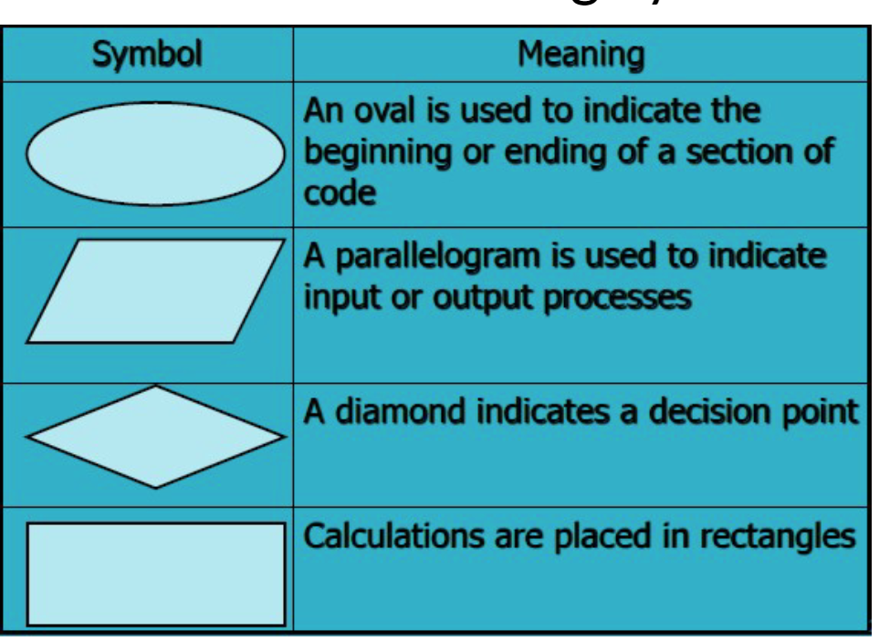
Flowcharts

graphical approach to creating a coding plan

Epecially appropriate for planning large or complicated programming tasks

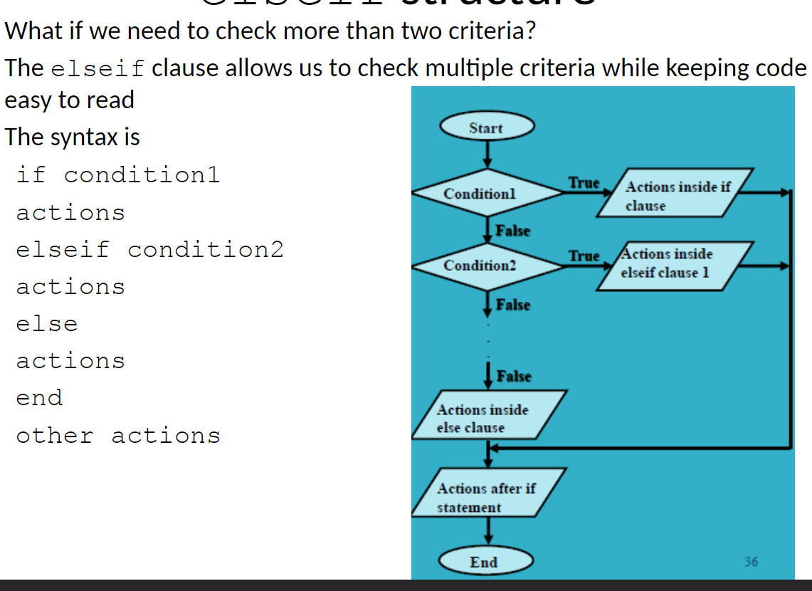
if statement

allows us to execute a series of statements if a condition is true and to skip those steps if the condition is false

can add else statements and if else

Nested if statements

If statements can be nested within each other

Allow you to choose 2 parameters of interest

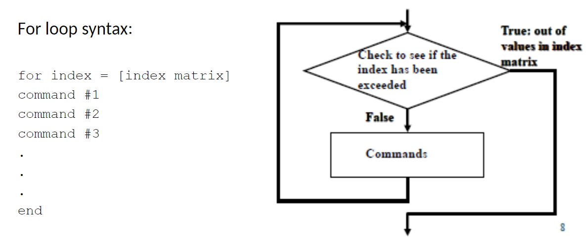
for loop

repeat a block of commands for a specified matrix which is known before the loop is executed

indexed

one loop _ be written inside another loop

one loop CAN be written inside another loop

Called a nested loop

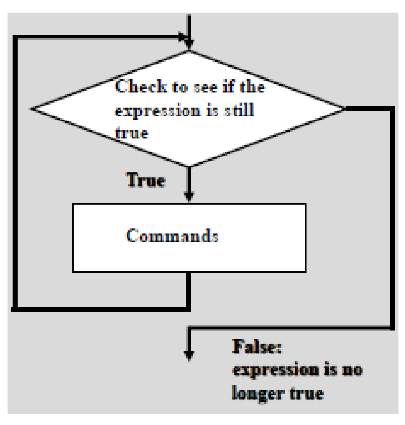
while loops

Loops are MATLAB constructs that allow a sequence of MATLAB statements to be executed more than once

loops repeat a block of commands as long as an expression is true (1)

The loop ends when the expression is false (0) and any code following the loop (after the end) is then executed

useful for repeating a procedure an unknown number of times as long as a certain statement is true

can be used to acquire data in experiments

useful when a procedure needs to be repeated until a specific criterion is met

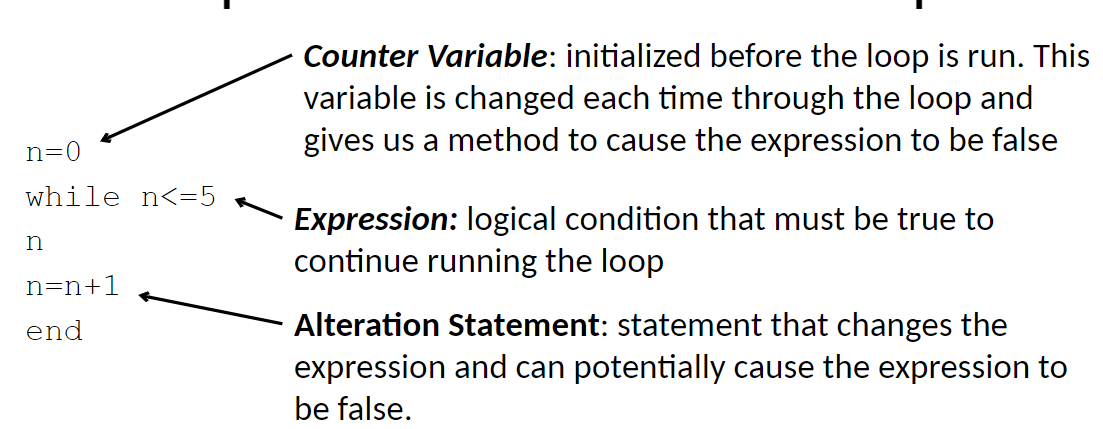
Components of a while loops

Built-in timer function

tic toc

tic starts the timer

time elapsed since the timer was started is given by the built-in function toc

Writing Functions

• function [output1 output2] = function_name(input1, input2, input3)

  • output1 = equation using inputs

  • output2 = equation using inputs

• end

Data import/Export

• uiimport(name)

• xlsread(‘filename.xls’) - in matlab folder, read excel

• xlswrite(‘filenamr.xls’, M) - writes array M into excel

• load <filename>

Exponential Growth

population & linear growth, compound interest

Increasing, asymptotic to the left

y=Ce^kt

Exponential Decay

radioactive decay, depreciation, fluorescent decay, learning, sales, stress

y=C(1-e^-kt)

y=Ce^-kt

Logarithmic Growth

population growth with limiting factors, acidity, sound, sigmodal curve

y=1/(1+be^-kt)

y=a+b*ln(t)

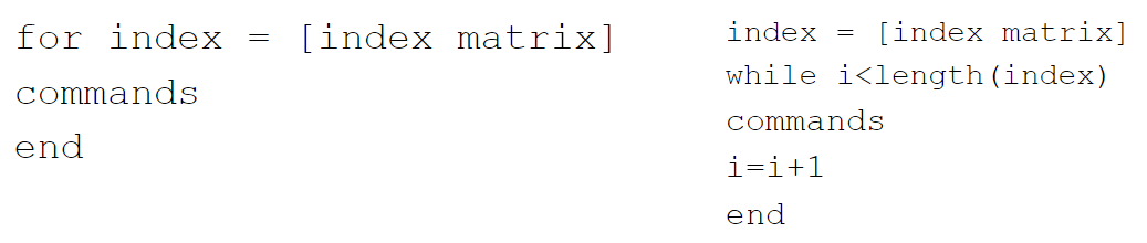
Converting a for loop into a while loop

One can change any program written with a for loop into a program written using a while loop instead

Change the index matrix of the for loop into an expression or set of variables that can be used in the while loop

for index → i=0

while i<length(index);

commands;

i=i+1; end

Converting a while loop into a for loop

while expression →

for index=data;

if expression break;

end;

commands;

end

Text File Types

1. Binary - fast, complicated, “native” format, .xls, .doc, .mat

2. ASCII - matlab, text editor, simple, .txt, .dat, .cvs

break statement

can be used to terminate a loop prematurely

cause termination of the smallest enclosing loop

How to improve loop efficiency

pre-allocating space for a placeholder variable before entering the loop

Command to display text and matrix values

fprintf()

Different place holders for fprintf

Need in the format-string in order for variable to show up in your display on the command window

%d - integer notation

%f - fixed point notation (decimal)

%e - exponential notation

%g - whichever is shorter between %f or %e (insignificant zeros do not print)

%c - character information

%s - string of characters

normal distribution/gaussian

a probability distribution that is symmetric about the mean, showing that data near the mean are more frequent in occurrence than data far from the mean. In graphical form, it appears as a "bell curve"

trapz(y)

MATLAB function for trapezoidal area under the curve

Normal Probability Plot

x values vs. z values or normplot(x)

right skew - plot bends up and left

left skew - plot bends down and left

short tail - less variance than expected

long tail - more variance than expected

What is the area of a normal curve within 1 standard deviation (between μ+σ and μ-σ)

68%

What is the area of a normal curve within 2 standard deviations (between μ+2σ and μ-2σ)

95%

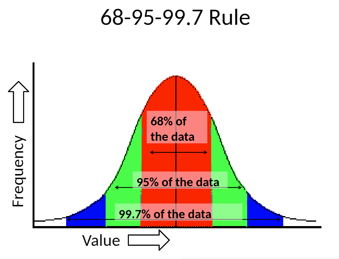
What is the area of a normal curve within 3 standard deviations (between μ+3σ and μ-3σ)

99.7%

Code for a gaussian distribution

f(x) = gaussmf(x, [std mu])

std is the standard deviation

mu is the mean

x is the parameter under scrutiny

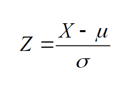
The standard normal distribution (z)

All normal distributions can be converted into the standard normal curve by subtracting the mean and dividing by the standard deviation

The probabilities given the z is in a table

_ continuous random variables are normally distributed

NOT ALL continuous random variables are normally distributed

How to tell if your data is normally distributed

1. Look at the histogram! Does it appear bell shaped?

2. Compute descriptive summary measures—are mean, median, and mode similar?

3. Do 2/3 of observations lay within 1 std dev of the mean? Do 95% of observations lay within 2 std dev of the mean?

4. Look at a normal probability plot—is it approximately linear?

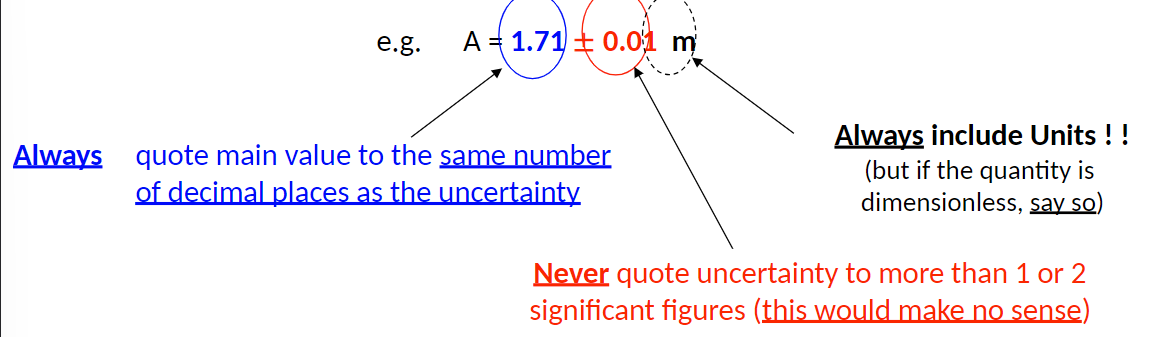
Every physical quantity has:

A value or size

Uncertainty (or Error)

Units

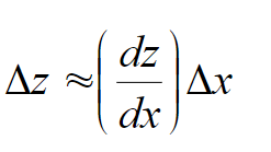
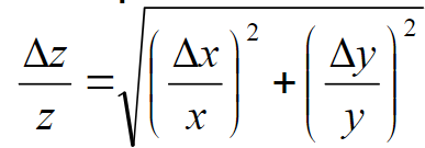
Error propagation equation to the first order if (∆x)/x is small:

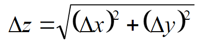
Equation for error propagation with addition and subtraction

Equation for error propagation with multiplication and division

Result Formats

numeric value +- error margin units

• floating point - scientific notation

• rational - exact result

• numeric - normal, general result

Errors in computational models

Those due to uncertainty in the formulation of the mathematical models and deliberate simplifications of the models

Caused by rounding, data uncertainty, and truncation

Truncation Errors

Results from using an approximation in place of an exact mathematical procedure

The difference between analytical and numerical solutions

Reasons for Math Modeling

1. Import meaning to data

2. Help obtain data

3. Help solve for specific conditions

Analytical Model

full mathematical solution

Numerical Model

Eulers, new value = old value + slope*step size, finite difference

Zero Order vs First Order vs Second Order

0: no change

1st: Linear change with change in x

2nd: Quadratic change with change in x

Any smooth function can be approximated as a

Polynomial

As the degree of the polynomial approximation _ the _ accurate the approximation

As the degree of the polynomial approximation INCREASES the MORE accurate the approximation

(adding more terms reduce truncation error)

Model Error

Incomplete mathematical models

e.g: E=mc²

Techniques to solve for roots

1. Graphically - rough and inaccurate

2. Trial and Error (using excel) - long winded

3. Automated methods (require an initial guess)

   1. Bracketing Methods - Robust

      • 2 initial guesses that “bracket” the root

   2. Open methods - Faster

      • 1 guess or more but no need to bracket

2 types of solutions for root finding

1. Implicit (cyclic)

2. Explicit (one specific solution)

Bracketing techniques for root finding

1. Incremental Search

   • Can work

   • Very inefficient

2. Bisection Method

3. False Position Method

Bracketing Bisection Full Process

• Given upper and lower bounds (xl and xu)

• [ determine xr, value halfway between xl and xu

• Calculate f(xr)*f(xl) and f(xr)*f(xu), or only one if a root is guaranteed

• A negative value determines the side the root is on. 

• f(xr)*f(xl) = -#, root on the left; f(xr)*f(xu) = -#, root on the right

• Left: xr becomes xu. Right: xr becomes xl ]

• Repeat bracketed until required degree of precision is met

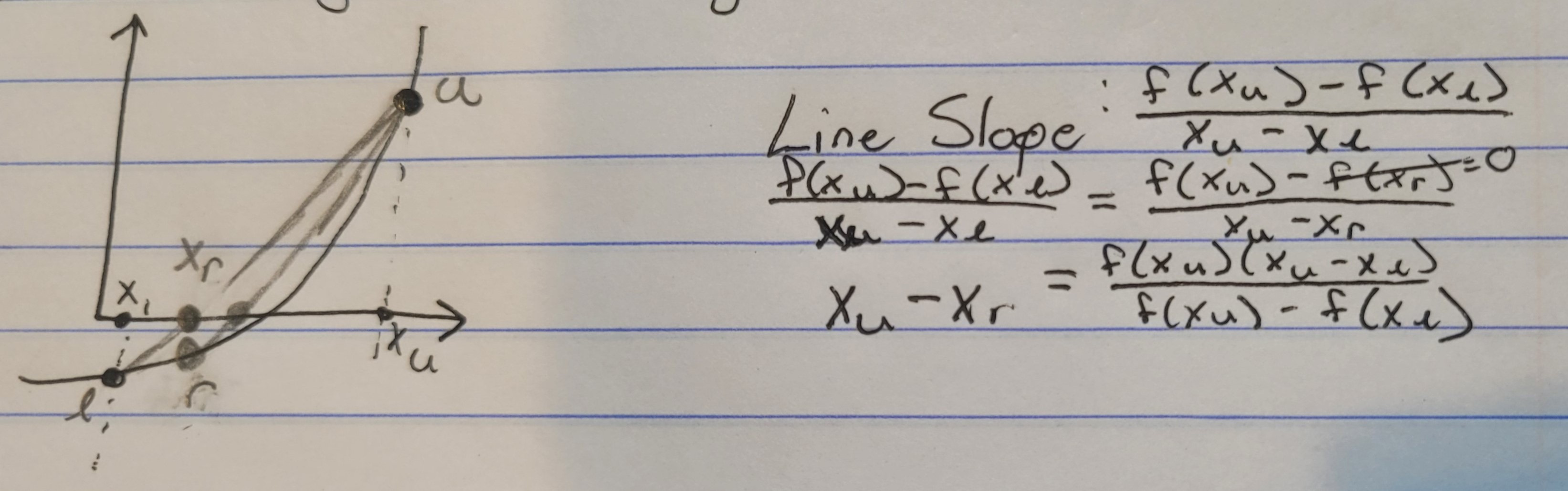
False Position Method

• Linear interpolation, root finding

• Joins F(xl) and F(xu), intersection of line with x-axis = root estimate

• Slope = [ F(xu) - F(xl) ] / [ xu - xl ] =>  [ F(xr) - F(xl) ] / [ xr- xl ]  or xl -> xr

  • xu-xr = [ F(xu)*(xu-xl) ] / [ F(xu) - F(xl) ]

• Issues: multiple roots, one fixed point, poor convergence for high curvature

• faster than other bracketing methods, robust

Steps of False Position Method

1. Start with 2 values that bracket a singular root, L and U

2. Calculate slope between the to points (draw line)

3. Where the line crosses the x axis is the x value for R (slope line y=0)

4. Find the correlating y value for the X_r on the function line

5. Last step:

   • If Y_r = 0 done

   • If Y_r * Y_l = pos replace L with R and repeat

   • If Y_r*Y_l = neg replace U with R and repeat

Open Methods Overview

• fast

• divergence issues sometimes

• when they do converge they do so more quickly

• require 1 starting value

• 3 possible results

  • Diverge

  • Converge Overdamped

  • Converge Underdamped

• Types

  • Fixed point iteration

  • Newton Raphson

Overdamped (Convergence)

logarithmic like plot gradually approaching actual value

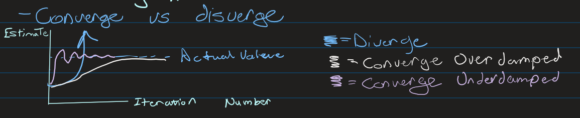
Underdamped (Convergence)

oscillate around actual value with slowly decreasing amplitude

Diverging (Convergence)

points away from actual value and gets further away over time

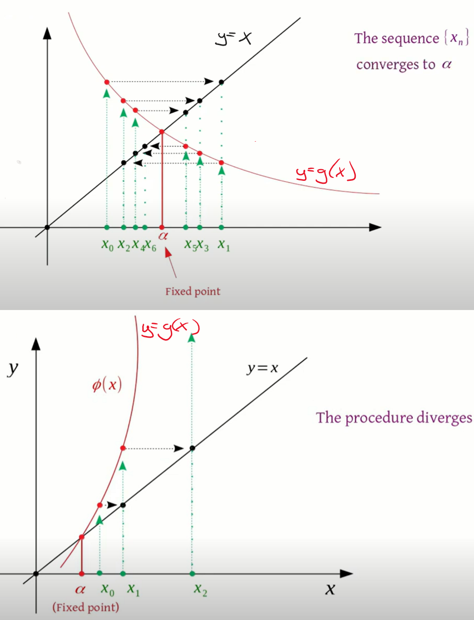
Fixed Point Iteration

• Root finding open method

• Rearranges function f(x)=0 to x=g(x)

  • done with algebraic manipulation or log or simply adding x to both sides

• We use this to create a formula that predicts a new value of x as a function of a previous value

  • x(i+1) = g(xi)

• Relative error = Ea = | [ x(i+1) - xi ] / x(i+1) | * 100%

• Plot the x vs. g(x). Point of intersection = root

• Spiral convergence or divergence

• x0 -> g(x0) -> x=g(0) at x1 -> x1 -> etc.

Fixed point Iteration Visualized

Plot the x vs. g(x). Point of intersection = root

Newton Raphson

• Most widely used root finding method

• Initial guess xi, extend tangent from the point [xi, F(xi)]

• Point where tangent line crosses x-axis becomes improved estimate

• F’(xi) = F(xi) / [ xi - x(i+1) ]

• Fastest convergence, very efficient

• Bad for: multiple roots, high curvature, local minima, sigmodal curves

  • Can have divergence or jumping between roots

  • Local min / max send estimate to - or + infinity lkk

• x(i+1) = xi - F(xi)/F’(xi)

• Backwards/Secant: x(i+1) = xi - F(xi) * [ xj - x(j-1) ] / [ F(xj) - F(xj-1) ]

MATLAB Root Finding

• fzero(function, guess) → fzero( @x x²-9, 4)

  • Combo of bisection, secant, and inverse quadratic interpolation

  • can have guess as an interval [0 4] for positive roots

• Polynomial - r=roots(c)  being a row matrix of the coefficients of the equation

• Opp: poly(r) = coefficients

Measuring Slope

• Forward Difference 

  • Slope = [ F(i+1) - F(i) ] / [ x(i+1) - x(i) ]

• Backwards Difference 

  • Slope = [ F(i) - F(i+1) ] / [ x(i) - x(i+1) ]

• Centered Difference

  • Slope = [ F(i+1) - F(i-1) ] / [ x(i+1) - x(i-1) ]