MTH 267 - Differential Equations Module 6 (Ch.7)

Transforms

operations ‘transforms’ 1 function into another

e.g. derivatives, integral

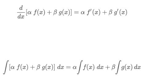
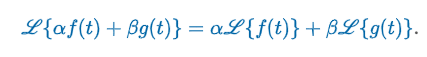
Linearity Property

“L operating on a linear combination of two differentiable functions is the same as the linear combination of L operating on the individual functions”

Definite Integral

A definite integral of f w.r.t. 1 variable leads to a function of the other variable

e.g. transform function f of the variable t into a function F of variable s

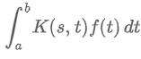
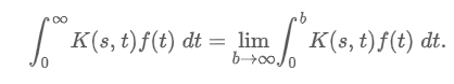
Integral Transforms

“Interval of integration is the unbounded interval [0, ∞). If f(t) is defined for t ≥ 0, then the improper integral is defined as a limit”

• Convergent: limit & integral DOES exist

• Divergent: limit & integral does NOT exist

Kernel

k(s, t)

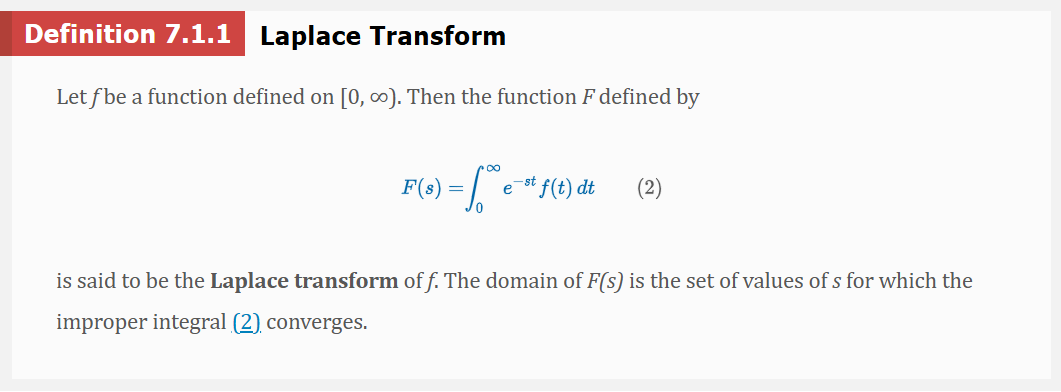
Laplace Transform

Note: also denoted as ℒ{f(t)}

Application: use a lowercase letter to denote the function being transformed and the corresponding capital letter to denote its Laplace transform

ℒ{f(t){ = F(s)

ℒ{g(t){ = G(s)

ℒ{g(i){ = I(s)

Shorthand limit notation

lim_b→∞()|₀^b become |₀^∞

Linear Transform

“Suppose the functions f and g possess Laplace transforms for s > c₁ and s > c₂ , respectively. If c denotes the maximum of the two numbers c₁ and c₂ then for s > c and constants α and β we can write…”

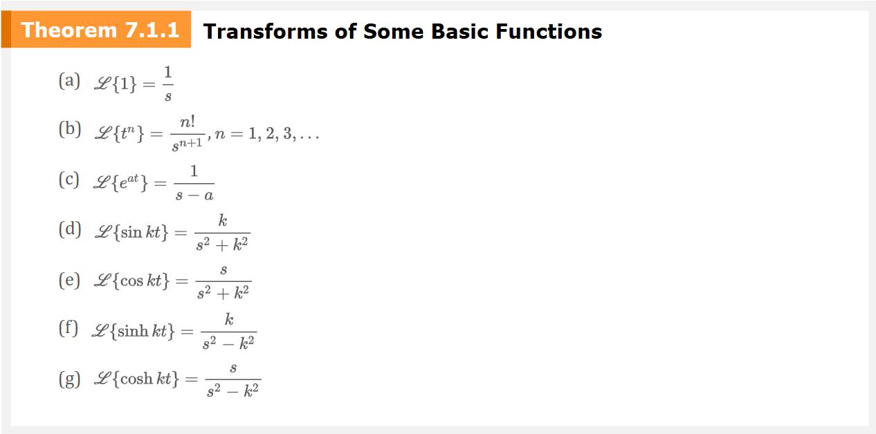
Transform of Basic Functions

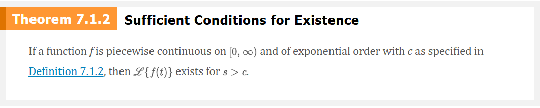
Existence of ℒ{f(t)}

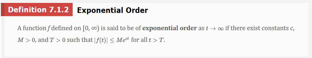
“ Sufficient conditions guaranteeing the existence of ℒ{f(t)} are that f be piecewise continuous on [0, ∞) and that f be of exponential order for t > T.”

Exponential Order

If f is an increasing function, then the condition |f(t)| ≤ Me^ct for all t > T simply states that the graph of f on the interval (T, ∞) does not grow faster than the graph of the exponential function Me^ct , where c is a positive constant.

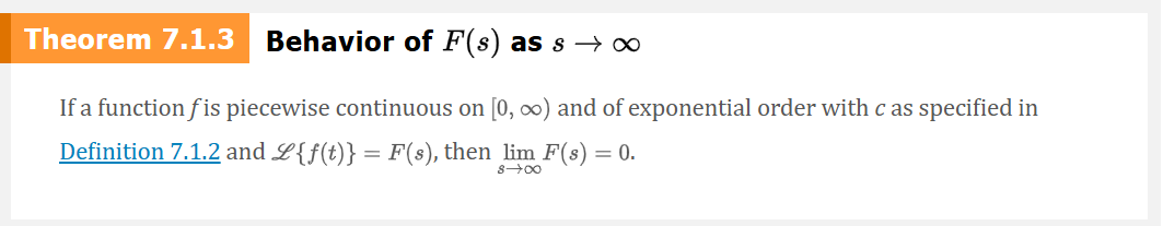
Behavior of F(s) as s → ∞

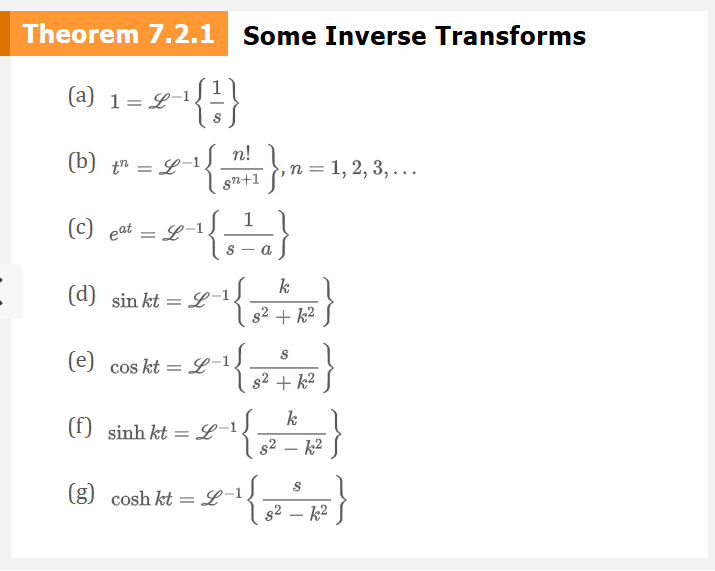
Inverse Laplace Transforms

Since ℒ{f(t)} = F(s), then f(t)=ℒ^-1{F(s)}

Some Inverse Transforms

Linearity of the Inverse Laplace Transform

“Suppose the functions f(t)=ℒ^-1{F(s)} and g(t)=ℒ^-1{G(s)} are piecewise continuous on [0, ∞) and of exponential order. Then for constants α and β we can write…”

Transforms a Derivative Proof

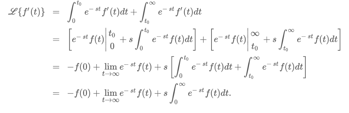
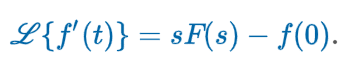
Transforms 1^st Derivative

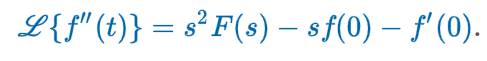
Transforms 2^nd Derivative

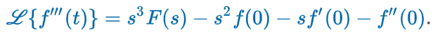
Transforms 3^rd Derivative

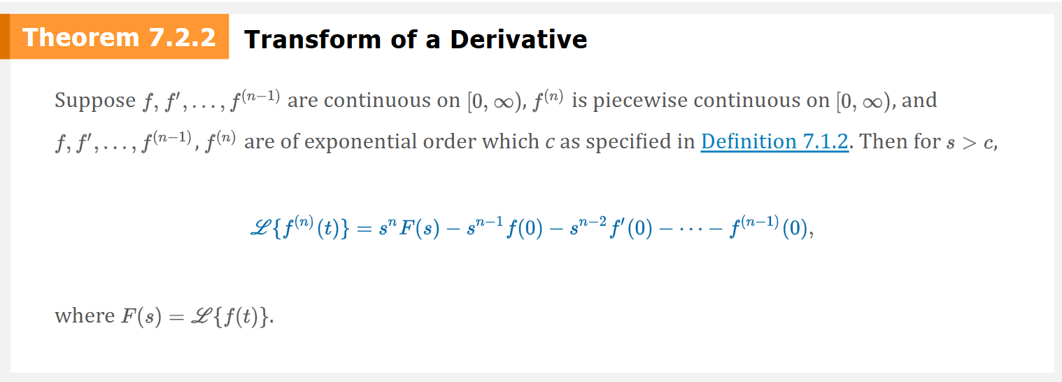
Transform of a Derivative (Theorem)

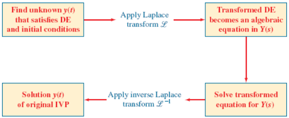
ODE w/ Laplace Transforms

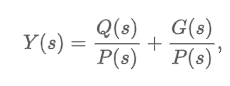
The Laplace transform of a linear differential equation with constant coefficients becomes an algebraic equation in Y(s).

• P(s) = a_nsⁿ + a_n-1s^n-1 + … + a₀

• Q(s) = polynomial in s of degree less than or equal to n - 1 consisting of various products of the coefficient, a₁, i = 1, …, n and the prescribed initial conditions y₀, y₁, …, y_n-1

• G(s) = Laplace transform of g(t)

y(t)=ℒ^-1{Y(s)}

Steps in solving an IVP by the Laplace transform