SOA Exam P Probability Distributions

Bernoulli Trial

An experiment in which there are exactly two possible outcomes

Binomial distribution

A random variable X represents the number of successes observed from the n Bernoulli trials

Binomial Parameters

n = number of trials

p = probability of success

q = 1-p

Binomial probability function (f(x))

E[X] binomial function

E[x] = np

var(x) binomial function

var(x) = npq

MGF binomial function

Additive property of binomial function

Sum of independent binomially distributed variables each with probability p, has parameters of p and the sum of all n

Negative binomial distribution

X is the number of failures before r successes in a series of independent Bernoulli trials

Negative binomial parameters

r = desired number of successes

x = number of failures before r successes

p = probability of success

q = 1-p, probability of failure

Negative binomial probability density function f(x)

f(x) = Pr(X=x) = (r + x - 1)!/x!(r-1)! * p^r * q^x

Expected value of negative binomial distribution E[X]

E[X] = rq/p

Variance of negative binomial distribution var(x)

var(x) = rq/p^2

Moment generating function negative binomial distribution

Mx(t) = ((1 - qe^t)/p)^-r

Additive property of negative binomial distribution

If Xi follows a negative binomial distribution with parameters ri and p, and they are independent, then the sum of them follows a negative binomial distribution with parameters as the sum of the ri and p.

Geometric distribution

The number of failures observed from the series of Bernoulli trials until the first success occurs

Parameters of geometric distribution

p = probability of success

q = 1-p

x = number of trials before first success

Probability density function of geometric distribution

f(x) = Pr(X=x) = q^x * p

Probability mass function of geometric distribution

F(x) = Pr(X <= x) = 1 - q^x+1

Expected value of geometric distribution

E[x] = q/p

Variance of geometric distribution

var(x) = q/p^2

MGF of geometric distribution

Mx(t) = ((1 - qe^t)/p)^-1

Additive property of geometric distribution

A sum of n independent geometric distributions with parameter p follows a negative binomial distribution with parameters r = n and p.

Hypergeometric distribution definition

X is the number of Type 1 objects in a sample of n objects randomly selected without replacement from a population of m objects, of which m1 are type 1 and m2 are type 2 (where m = m1 + m2.

Hypergeometric probability distribution function

f(x) = Pr(X=x) = C(m1,x) * C(m2,n-x) = C(m,n)

Expected value of hypergeometric function

E[x] = nm1/m

Variance of hypergeometric function

var(x) = n(m1/m)(m2/m)((m-n)/(m-1))

Definition of poisson distribution

X is the number of occurrences of some "rare" event in a unit time period where λ is the rate of occurrences per unit time period

Probability distribution function

f(x) = Pr(X=x) = e^-λ*λ^x/x!

Expected value of a poisson distribution

λ

Variance of poisson distribution

λ

MGF of poisson distribution

Mx(t) = e^(λ((e^t)-1))

Additive property of poisson distribution

Sum of poisson distributions has parameter of the sum of all the λ

Uniform distribution

Constant probability density function on the interval [a,b]

PDF of uniform distribution

f(x) = 1/(b-a)

CDF of uniform distribution

F(x) = (x-a)/(b-a)

Expected value of uniform distribution

E(x) = (b+a)/2

Variance of uniform distribution

var(x) = ((b-a)^2)/12

median of uniform distribution

m = (b+a)/2

MGF of uniform distribution

Mx(t) = (e^bt - e^at)/t(b-a)

exponential distribution parameters

θ

Exponential distribution CDF

F(x) = 1-e^(-x/θ)

Expected value of exponential distribution

θ

variance of exponential distribution

θ^2

median of exponential distribution

m = θ*ln(2)

moment generating function for exponential distribution

M(t) = 1/(1-θt) for t < 1/θ

memoryless property for exponential distribution

Pr(X > x0 + x | x > x0) = Pr(X>x)

Exponential distribution PDF

f(x) = (1/θ) e^(-x/θ)

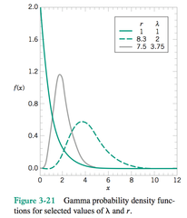
Gamma distribution

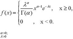
Gamma distribution function

expected value of gamma distribution

E[x] = αθ

variance of gamma distribution

var(x) = αθ^2

moment generating function of gamma distribution

M(t) = 1/((1- θt)^α)

Additive property of gamma distribution

Sum of gamma distributions has parameters of the sum of the α and θ.

Normal distribution expected value

μ

Normal distribution variance

σ^2

The central limit theorem

If X1...Xn are independent and identically distributed with mean μ and variance σ^2.

For large n, then the sum of X1...Xn is approximately distributed with mean nμ and variance nσ^2. The mean of all of them is distributed with mean μ and variance σ^2/n

Joint probability function

Pr(X=x and Y=y) = fxy(x,y)

Conditional probability function of X fx(x)(multivariate)

fx(x|Y=y) = fxy(x,y)/fy(y)

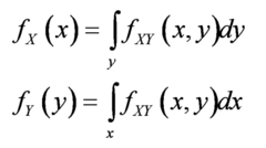
Marginal probability density function of X

E[g(x,y)]

sum or integral of g(x,y)fxy(x,y)

Mx,y(s,t)

E[e^sX+tY]

cov(X,Y)

E[XY] - E[X]E[Y]

Covariance function properties

var(X) = cov(X,X)

cov(X,Y) = cov(Y,X)

cov(aX + bY,z) = a cov(X,Z) + b cov(Y,Z)

cov(X,Y) = 0 if X and Y are independent

var(aX + bY) = cov(aX+bY,aX+bY) = a^2 var(X) + b^2 var(Y) + 2abcov(X,Y)

Correlation coefficient

rho

cov(X,Y)/sd(X)sd(Y)

bivariate normal distribution conditional distribution of x

E[X|Y=y] = μx + ρ(σy/σx)(y-μy)

var(X|Y=y) = σx^2(1-ρ^2)