Topics in Macroeconomics - theory

is GDP larger for a bigger economy?

• yes

does economic welfare grow with GDP per worker?

• usually yes

• it also depends on the income distribution

important aspects of value added that GDP does not measure

• much of non-market value added such as house production and subsistence farming

• there are attempts to estimate the value of government services such as the NHS

• much of the underground economy: illegal markets transactions (eg buying and selling of drugs) and legal yet unreported market transactions (eg vinted)

• there are imperfect ways to assess unreported income, but some are not captured

• much of the change in natural resources (eg stock of minerals, air quality, soil fertility)

• eg production of oil is counted but not the stock of oil remaining in the economy

• many services that are provided free of charges (eg Wikipedia)

• pollution, leisure, life expectancy, inequality, crime, and freedom are incorporated imperfectly, if at all, in GDP

important issues of GDP

• GDP is an aggregate measure so it is silent about inequality (does not discuss about income distribution)

• GDP measures the economy’s production, not its consumption (consumption of goods and services is what we actually care about)

• GDP does not coincide with gross national income (GNI) (it does not measure income properly as it does not include consumption; only measures production)

• GDP is not a accurate measure for market values of goods and services for a less competitive economy as the market prices are off/don’t exist

• therefore, GDP is only a valid measure if there exists reasonable competition between producers

supply and demand notations

• qs = the economy produces some quantity of sector s goods (supply)

• ms = the economy imports an additional quantity of sector s goods (supply)

• ds = good s is used for domestic consumption (demand)

• xs = good s is used for exports

• bs = good s is used as an intermediate good

• ps = price of good s (both the price that producers charge and users pay; we assume there is no difference

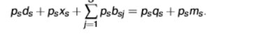
intermediate goods equation

• the intermediate good from sector s is potentially used by all industries of the economy

demand and supply equation

• domestic consumption ds = cs + gs + is could be further decomposed into private consumption, government consumption, and investment

why can’t we just use the gross output of goods for calculating the production of economy?

• some of the goods that we made will be intermediate goods for production of further goods

• when firms are using intermediate goods, this does not mean they are producing something new; just buying something from another source

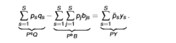
equation of the value of demand and the value of supply

• we are multiplying everything at the sector level by price

• LHS = demand

• RHS = supply

• psqs =Y (GDP)

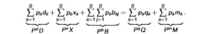
equation for aggregated accounting identity

• summing over all sectors s yields an aggregated accounting identity

• aggregated price indexes are constructed from the individual ones

• the capitalized prices indicate price indices of the underlying quantity indices

why do we take out intermediates when we calculate value added?

• so they are not double counted

• if we did not take away the intermediate goods, it would lead to misleading values of production

• it would make it seem like a company is producing a lot

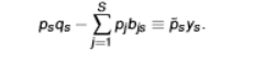
value added of sector s equation

• the value of sales minus the cost of the intermediate goods

summing over all the value added of sectors in an economy allows us to obtain….

• … nominal GDP

• the distinction between nominal and real GDP is because the same thing can cost different amounts in different places

• right now, we don’t know what the differences are

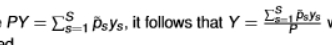
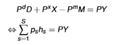
equality between final demand and GDP + imports

• we obtain this from replacing P^qQ - P^bB from the aggregated accounting identity into the nominal GDP equation

• so we go from P^dD + P^xX + P^bB = P^qQ + P^mM to what is in the picture

is real GDP a price or quantity index?

• quantity index

real GDP equation

• the price index P must be somehow defined

• can use GDP deflator

• it is more tricky to compare countries’ real GDP as there are many sectors and there simply does not exist a single aggregate quantity Y

• real GDP can also be computed as Yi = Zi/Pi where Pi = aggregate price index and Z = the sum of price*quantity of all the goods the economy produces

real value added (expenditure side)

• the first equation could be rewritten as: P^dD + P^xX = PY + P^mM

• hs = ds + xs - ms

• as hs represent actual real quantities (eg a kilo of apples), it is easier to construct a price index P (and therefore a real GDP index Y) from the expenditure side

difference between the production side and expenditure side of GDP

• for the production side, we talk about value added, which is a hard thing to measure

• for example, how do we calculate the value added inside a business?

• the production side only exists as an accounting concept

• for the expenditure side, we are talking about the final usage in the economy, they are actual real quantities

• therefore, we are able to count them all and see the prices at which those things were traded at

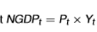
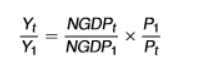
nominal GDP formula

• as the index is t, we are measuring across time

• we would change the index to i if we are measuring across countries

real GDP growth formula

• 1 is the base year

• P1/Pt is the ratio of the GDP deflator

• as the index is t, we are measuring across time

• we would change the index to i if we were wanting to measure across countries

• real GDP growth from period 1 to period t depends on P1/Pt (GDP price deflator)

what does the GDP deflator rely on?

• it relies on a suitable construction of P by national statistics offices

• if we ignored this, then a general increase in prices (inflation) would imply growth in real GDP

how do we compute NGDPi for measuring real GDP across countries?

• national statistics offices compute NGDPi in each country

• it can be translated into a common currency such as US dollars

is it easy to compare prices across countries?

• no

• due to data availability (or unavailability)

• not all countries have readily available information of the prices of goods

• the construction of an index P is more arbitrary

why is the nominal GDP relatively higher in rich countries?

• because the price level is higher in rich countries

number of workers formula

• we write it as working age population/population as we are expressing it as a ratio of the total population

• a country will tend to have more workers if its share of the working age population is high (ie low share of people younger than 16 years)

working population in rich and poor countries

• poorer countries typically have a lot of young children

• rich countries, such as Japan, have an opposite skewed pyramid where they have a lot of retired people so they are not within the working age population anymore

• more of the population is working in richer countries and a reason for this is due to higher female participation in work

employment rate formula

• the employment rate is only computed from the working age population

• it depends on the labour force participation rate and the unemployment rate

• participation rate depends on the willingness to work in the market sector

• the participation rate can vary substantially for the young (alternative = education), the old (alternative=retirement), and women

why is relative GDP per capita slightly higher in rich countries?

• mostly because the worker to population ratio is slightly higher in rich countries

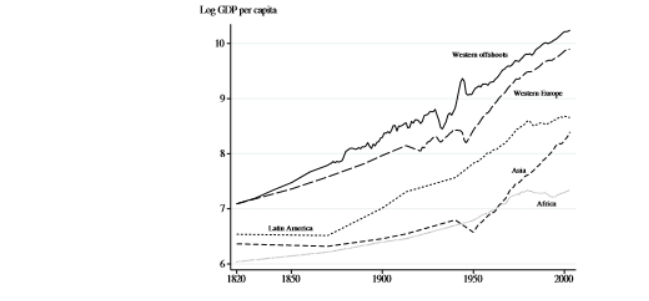
stylized facts regarding GDP growth and levels

• economic growth is a recent phenomenon, it takes off around 1800 (industrial revolution) in Western Europe and its offshoots

• over the last century, growth picks up around the world especially in Asia

• over the last two centuries, the evolution of the industrial leaders UK and the US can be approximated by a straight line (in logs this implies a constant average growth rate)

• the relative level of GDP per worker in 1960 is a good predictor of the relative level of GDP per worker in 2000

• log GDP per worker in 1960 cannot predict future growth rate

• this tells us that growth rates are unpredictable based on initial income

• countries do differ significantly in growth rates, but this is not systematically related to the initial level of GDP per worker on average

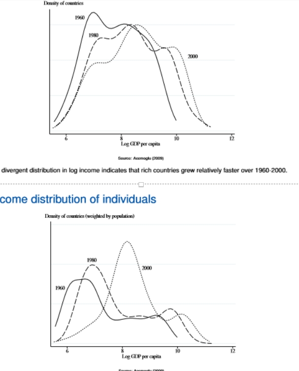
world income distribution of countries and individuals

• a slightly more divergent distribution in log income indicates that rich countries grew relatively faster over 1960 -2000

• peaks have changed over time

• when countries are weighted by population (of individuals) there is evidence of slight convergence (eg China and India which have a larger weight attached to them)

• we have moved from poorer levels to a more middle ground

• this proves that countries have driven themselves out of extreme poverty and managed to achieve high levels of economic growth

why have western offshoots achieved high economic growth when Latin American has not, despite both starting off as colonies? (can link this to misallocation)

• a lot of governing institutions in Western offshoots were modelled based of the UK (similar to their country of origin) - inclusive institutions

• a lot of US government system and law is based off the UK

• white colonists tended to stay in these western offshoots (eg US and Australia) which allowed this to happen

• this created the climate of economic growth to take place

• these institutions created the environment for market economy to flourish

• in latin america, the institutions were created purely to extract resources of the country (extractive institutions)

• created an economy where the colonists governed and forced the natives to work for them

• the natives would produce wealth that the colonists would take back to their country of origin

• they did not have secure institutions to allow the climate for economic growth to flourish

• political and economic instability can be traced back to these historical moments

is there convergence in GDP per capita across countries?

• there is large divergence between countries from 1800 to 1950

• since then until 2000, quite stable on average with some countries converging and others diverging

• slight divergence when countries are not population-weighted

• slight convergence when countries are weighted by population (China and India)

• on average, GDP seems to be growing (countries are becoming richer)

• countries around the world are converging but to their own steady-states, rather than to the frontier

how do we find that countries are converging to their steady states rather than to the frontier?

• if we condition on determinants of a country’s steady states (such as the investment rates in physical and human capital)

• we can see that countries below their steady states grow rapidly and those above their steady states grow slowly

key facts about GDP in the US economy

• for nearly 150 years, GDP per person has grown at a steady average rate of around 2% per year

• steady, sustained exponential growth

• the Great Depression resulted in GDP per person falling by nearly 20% in just 4 years

• not what we would expect as economic growth swamps economic fluctuations over a long period and the Great Depression was temporary

what cause the great divergence?

• the spread of growth over the very long run occurred at different points in time

the ratio of the richest country to the poorest country

• in 1300, the ratio was on order of 5

• in 1870, the ratio was on order of more than 10

• in 2010, the ratio was on order of more than 100

the reason why countries such as the UK, Germany, and France have lower incomes than the US

• they have lower GDP per hour worked

• ie not as productive

• although, western europeans tend to have higher life expectancy and lower consumption inequality

Jones and Klenow (2015) findings on growth and development

• western european countries like the UK and France have much higher living standards than their GDPs indicate

• while many rich countries are richer than we might have thought, the opposite is true for poor countries

• life expectancy and leisure tend to be lower, and inequality tends to be higher for poorer countries

has declining mortality raised consumption-equivalent welfare growth?

• yes and it has done so substantially

• notable exception being in the sub-saharan Africa

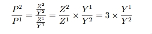
when we are computing the numerical value of the nominal GDP ratio between two economies, what should we take note of when making predictions?

• whichever economy produces more should have a larger GDP

• if the same economy also has higher prices, this will result in the overall price level being high which inflates the nominal GDP difference

• the ratio will therefore be higher than a plausible ratio of measured productivity/real income

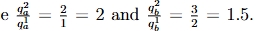
how do we compute the numerical values of the minimum and maximum plausible bounds of real GDP between two economies?

• we divide the quantity of each good produced in both economies like show in the picture

• whichever one is the lowest value is the minimum value (ie economy 2 is at least 1.5 times bigger than economy 1)

• whichever one is the biggest value is the maximum value (ie economy 2 is no larger than twice the size of economy 1)

• we calculate this in the ratio of Y2/Y1

using the formula for real GDP, how do we compute the numerical values of the minimum and maximum plausible price index bounds?

• real GDP formula: Yi = Zi/Pi so Pi = Zi/Yi

• Z2/Z1 is the nominal GDP ratio

• we replace Y1/Y2 by the inverse of the minimum and maximum plausible boundaries as we calculated for the boundaries for the ratio Y2/Y1 but now we have Y1/Y2

• this results in 1/Ymin and 1/Ymax

• we then multiply these figures by the nominal GDP ratio to get a plausible price index

• we could have also computed directly from the goods prices

• p2a/p1a and p2b/p1b where a and b are goods and 1 and 2 are economies

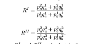
what is the difference between these two possible price ratios and what are the consequences of them?

• RI = the prices of one economy relative to the other are weighted by the goods quantities of economy 1 (quantities of economy 1 appears in both the numerator and the denominator)

• RII = the prices of one economy relative to the other are weighted by the goods quantities of economy 2 (quantities of economy 2 appears in both the numerator and the denominator)

• this means that index RI (RII) will tends to give more weight to the price difference of the good that is relatively important in economy 1(2)

• if economy 1 consumed only good a and economy 2 consumed only good b, RI would put all the weight on good a and RII would put all the weight on good b

• ie the indexes are biased in opposite directions

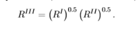
advantage of the fisher index

• if RI and RII are known to be biased in one or the other direction, the geometric average of the fisher index has the benefit to offer a middle between the extreme indexes

• using this ratio to compute the real GDP ratio will be different compared to using the nominal GDP ratio

• the fisher index takes into account the biasedness towards prices so this is why the factor will be different compared to the nominal GDP ratio

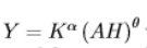
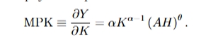
marginal product of physical capital using this production function

• just differentiate with respect to K

• MPK > 0 so this means that increasing K increases output

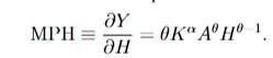
marginal product of human capital using this production function

• just differentiate with respect to H

• MPH>0 so increasing H increase output

how do we figure out the parameter restriction so that the marginal product of physical capital is strictly decreasing in K?

• we differentiate the marginal product of capital with respect to capital as for MPK to be strictly decreasing in K, dMPK/dK < 0

• this means that production is increasing and concave in K, which means that an increase in K will increase output but that the additional increase in output is getting smaller the larger K is

how do we figure out the parameter restriction so that the marginal product of human capital is strictly decreasing in H?

• we differentiate the marginal product of human capital with respect to human capital as for MPH to be strictly decreasing in H, we need dMPH/DH<0

• this means that production is increasing and concave in H, which means that an increase in H will increase output but that the additional increase in output is getting smaller the larger H is

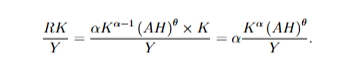
what is the factor income share of physical capital?

• we use the formula RK/Y where R = return to physical capital

• R = MPK

• as we know Y also equals the numerator, this means that the share of output earned by physical capital is α

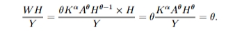
what is the factor income share of human capital?

• we use the formula WH/Y where W = return to human capital

• W = MPH

• Y again is equivalent to the numerator so the share of output earned by human capital is θ

what are the combined shares of income accruing to physical and human capital?

• their power inputs, ie θ + α

• the combined shares cannot be larger than 1 so the assumption that physical and human capital both earn their marginal product is only consistent as long as θ + α ≤ 1

• if θ + α <1, we have have that there is someone else (eg the firm or the owner of some unmodelled production factor such as land) who also obtains part of y

• if θ + α = 1, so θ = 1 - α, this implies the production function is Cobb-Douglas

• this means that physical capital earns a fraction α while human capital obtains the rest, 1- α

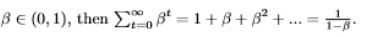
geometric series equation

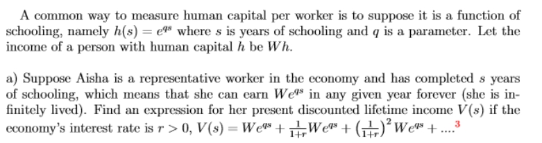
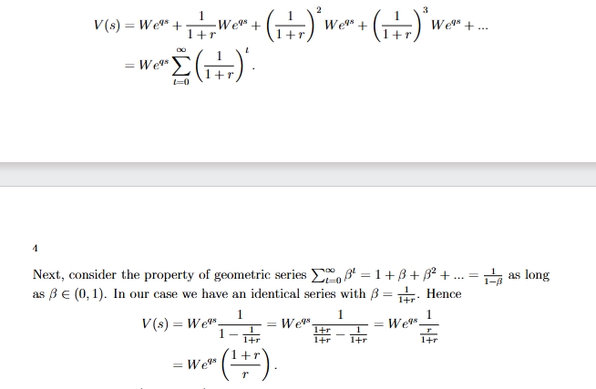
How do we answer this question about present discounted lifetime income using geometric series?

• we are getting all the flows and discounting the flows to get back to the start

• the geometric series will converge to some number (1/1+r)

• use the equation that is given and realise that the income is being compounded over multiple periods so each period applies the same discount factor of 1/1+r, meaning that this is to the power of t

• as 1+r/r = 1 +1/r, the present discounted lifetime income is decreasing in r

• this is because a higher interest rate means that future income is valued less from the present perspective

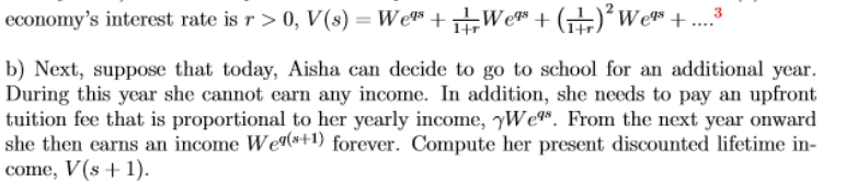
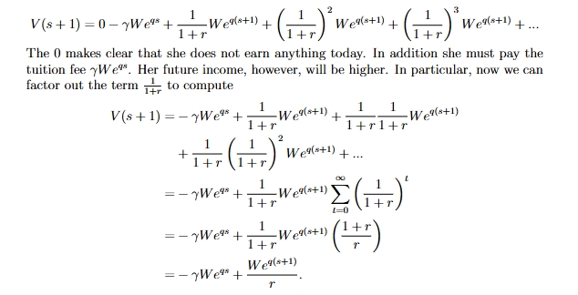
how would we compute the present discounted lifetime income if the individual can go to school for an additional year but during this year, she pays a tuition fee and earns no income?

• in the first period, the individual isn’t getting any income but she is paying for the tuition fee so this is why the first value is negative

• from period 2 onwards, she is earning some sort of income (this will be higher than if she had not had the extra year of schooling)

• we can factor out the term 1/1+r to compute her discounted lifetime income

• use the geometric series again when we find the sum of the interest rate

• the benefit of an extra year of schooling accrues in the future while today the individual only incurs costs

• a higher r requires a larger return to schooling

• a higher tuition fee requires the return to schooling to be higher in order to maintain the indifference condition

how can we find the value at which an individual is indifferent between two options?

• we must equate the two equations to each other

what do we do if we want to simplify an equation but we have the value e?

• we turn everything into logs

• the e will now end up as the power of it

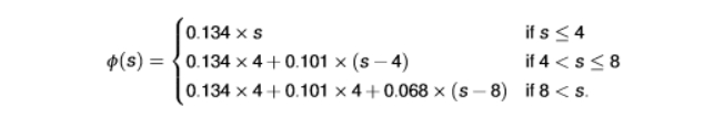
what does Caselli (2005) methodology express?

• the notion that an extra year of schooling is worth more in countries where educational attainments are low

• this is consistent with empirical estimates

• this shows that the percentage increase in human capital following an additional year of schooling depends on the actual years of schooling

• if the individual only has less than 4 years of completed schooling, the return is large: 0.134

• the returns decrease for those that have completed 4 to 8 years, and the lowest for those with more than 8 school years

when does log(1+x) ~ x?

• when x is ‘small’ in absolute value

• ie when it is between -0.1 and 0.1

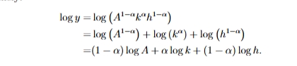
if we assume that k and h are exogenous, what is the elasticity of y with respect to A?

• the easiest way to do this is by taking logs

• separate each variable

• by taking the logs, we can put the powers of the variables infront of the logs

• whatever the power is, we multiply it out in logs

• dlogy/dlogA = 1 - α

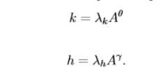
if we assume physical and human capital are just simple functions of A, what is captured if we assume θ > 1 and γ ∈ (0, 1)

• two production factors are not exogenous and are functions of technology

• when θ > 1 , the exponent is greater than 1, meaning capital increases at an accelerating rate as technology improves

• this means that k is increasing and is convex in A

• small improvements in technology (A) lead to disproportionately larger increases in capital

• in sectors where capital accumulation is highly responsive to technology (eg automation), technological progress has led to exponential growth in capital stock

• when 0<γ<1, the exponent is less than 1, meaning human capital increases at a decreasing rate as technology improves

• this means that h is increasing and is concave in A

• each additional improvement in A results in smaller and smaller gains in human capital

• human capital (ie skills, education) grows with technology but at a diminishing rate due to diminishing returns to education and training

Why will the elasticity that has k and h as endogenous variables be bigger than the elasticity that has k and h as exogenous variables?

• the second elasticity does not taking into account that A not only has a direct impact on y but also an indirect one through k and h

• the second elasticity just holds k and h constant

• the first elasticity assumes that changes in A also has an indirect (positive) effect on y through k and h, implying a stronger elasticity with respect to A

why do countries’ GDP differ?

• due to their stock of human and physical capital

Cobb-Douglas production function

• K = aggregate physical capital stock

• L = the number of workers

• h = human capital per worker

• alpha = factor share of capital (take values between 0 and 1)

• A = total factor productivity (TFP)

• as A is multiplied by labour, it is ‘labour-augmenting’/ ‘harrod-neutral’

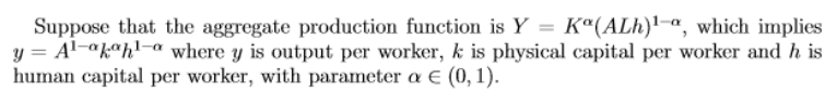
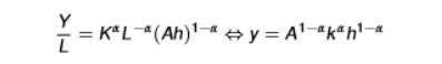
GDP per worker expression (including human capital)

• where y = Y/L (output per worker)

• where k = K/L (physical capital per worker)

properties of the cobb-douglas production function

• diminishing marginal returns to the three factors: K, L, and h

• this means that more of any single factor raises Y, but the effect becomes smaller as the factor increases

• constant returns to scale in K and L (or K and h), therefore doubling K and L (or K and h) doubles Y

why do we use the cobb-douglas production function if the aggregate production function not cobb douglas?

• they have reasonable properties, including roughly constant factor shares

• the properties are important in terms of long-term development as these factors will remain roughly constant over time

• theories suggest that certain short-term production functions resemble cobb-douglas in the long run (it matches with real data such as constant factor shares)

• simplicity

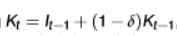
capital accumulation formula

• It-1 = what you have invested into the capital

• the second part is the capital left over from last period after depreciation

• t = period index (eg a year)

• I = investment

• delta = typical depreciation over the period

• we can reverse the equation and make the capital stock a series of investments made, taking into account the depreciation over time, but then we have to think about what was the initial capital stock (K0)

• It is reported in the national accounts across time so we only need to know K0 to construct the series

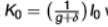
how do we calculate K0?

• we are assuming that the economy was on a balanced growth path before period 0

• g = growth rate of K

• in any case, if period 0 is sufficient far in the past, K0 will not matter much because most of it depreciates by t

• what matters is the sequences of investments made

how do we measure average human capital ‘h’?

• it is difficult to measure the level of skill of individuals

• it is instead proxied by schooling attainment as why would individuals go to school otherwise if it did not improve GDP per worker?

what do workers earn?

• w*h (assuming a competitive market

• where w = competitive wage (basic wage rate per labour unit) and h = human capital

• this means i can get the same wage for working half the hours if i have twice the human capital

• comparing individuals with different schooling attainments in a given economy (ie for a given w), one can infer the market value of human capital

human capital formula

• the power is a function of schooling in the economy s

• in many countries, the empirical relationship between earnings and an extra year of schooling is log-linear, suggestive of some constant multiplied by s (when we take the log, e disappears and we get the power multiplied by s in which the power becomes some constant)

• this means that 1 extra year of schooling increases wages by some constant %

• this constant is obtained from micro data

why in poor countries with low average schooling, a year of schooling procures larger gain (larger constant) than in rich countries?

• it is because there is a larger premium with going to high school in poorer countries; university is not so easily accessible

• this fact is important when comparing countries GDP per worker

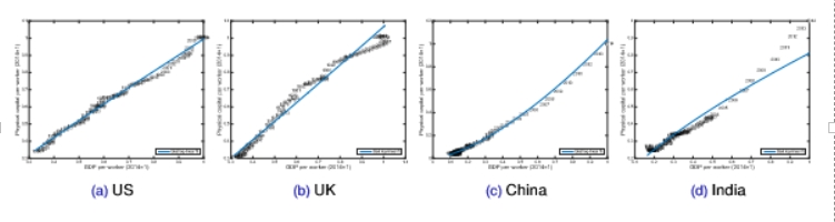
comments about physical capital and GDP across time, with selected countries

• computed from the regression logk = B0 +B1logy + e

• k = capital per worker, y = GDP per worker

• B1 for the US = 0.94, B1 for the UK = 1.05, B1 for China = 1.48, and B1 for India = 0.73

• in all countries, there is a strong positive correlation between k and y

• as China was getting richer, they were accumulating capital more than proportional (physical capital goes up by 1.5% for every 1% increase in income)

• there is a good line of fit which suggests that physical and human capital seem to relate with the income of country

• B1 =1 is a reasonable approximation

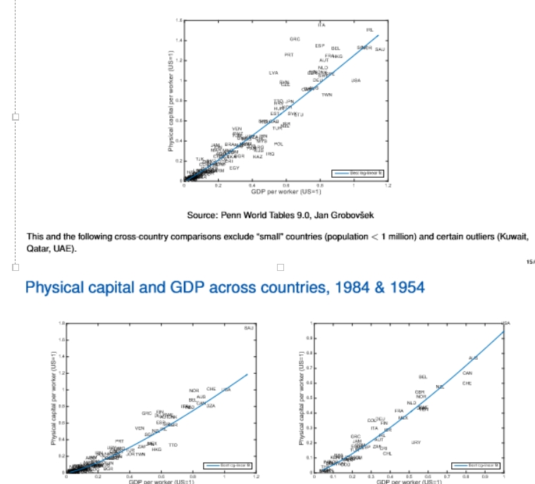
comments about physical capital and GDP across countries, 1954, 1984, and 2014

• top = 2014, bottom left = 1984, bottom right = 1954

• the relationship is logk = B0 +B1log y + e where k = capital per worker and y = GDP per worker

• B1 for 2014 = 1.11, B1 for 1984 = 1.28, B1 for 1954 = 1.24

• Since B1>1, we see that on average, richer countries have disproportionately more capital per worker than poor countries

• B1 = 1 is a reasonable approximation

• outliers include countries that have a large oil stocks such as Qatar, UAE, Kuwait

• if GDP per worker increases by 1%, capital increases by more than 1% (almost 1-to-1 relationship) (correlation, not causation!!)

• it is not free of noise/mismeasurement

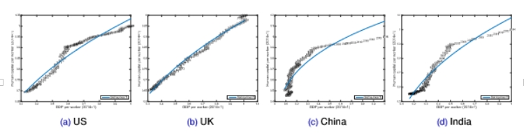
comments about human capital and GDP across time, selected countries

• we are considering the log-linear fit of log h = B0 + B1logy + e

• the estimated values of B1 are 0.35 (US), 0.36 (UK), 0.33 (China), 0.40 (India)

• for the above countries, we have a time series relationship with B1 = 0.35

• while human capital and GDP are positively correlated, the relationship is far from linear

• it is not a good fit for these countries, it is not linear but it is a positive relationship

• the correlation we observe is as follows: when real GDP per worker goes up by 3%, human capital increases by 1% (3-to-1 relationship)

• not trying to explain a causal relationship; we are looking at association between countries (as there is more income, there is more human/physical capital)

• we are looking at the reverse of the production function; what was the capital level when we produced the output?

• we are not trying to estimate the production function; these numbers have nothing to do with inside the production function

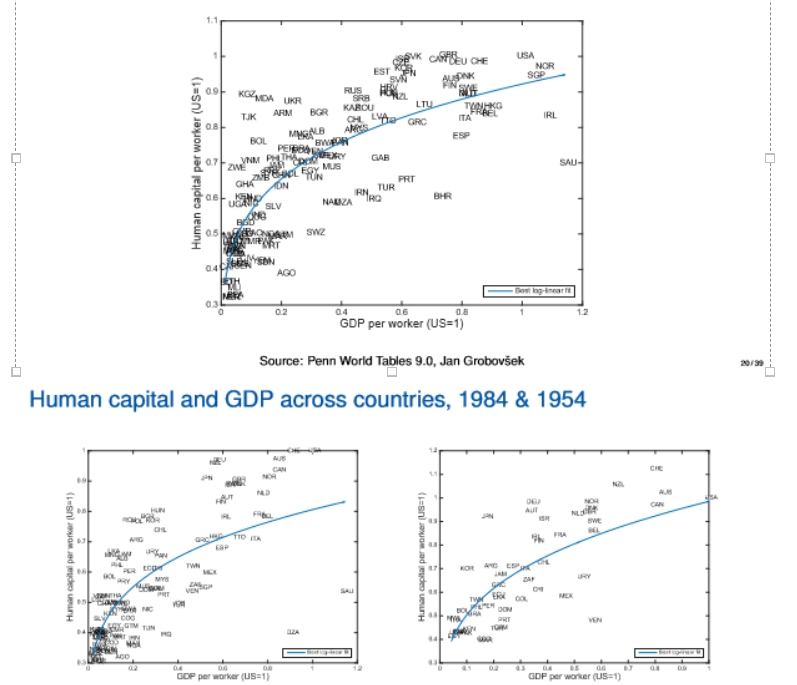
human capital and GDP across countries

• top = 2014, left = 1984, right = 1954

• we are considering the log-linear fit of log h = B0 + B1logy + e

• variables plotted in levels, not logs but if we estimate in logs, we get the bendy regression line

• means the relationship is not very strong

• the estimated values of B1 across countries are 0.21 (2014), 0.24 (1984), 0.29 (1954)

• since B1 ~ 0.25, this confirms that human capital per worker is a concave function of GDP per worker (shape we observe in the diagrams) - due to diminishing returns to human capital

• means that when GDP per worker increases by 1%, human capital increases by around 0.25%

• poor countries are relatively richer in human capital (relative to GDP)

• this means that as we are increasing income, we get less and less human capital (don’t have this relationship for physical capital)

• this is because as economies become richer, they can use automation instead of accumulate human capital, resulting in them substitute technology for certain labour functions => concave function

• when we observe an increase in GDP and human capital, there are other factors that are adjusting (omitted variable bias) - need to take into account all types of factors

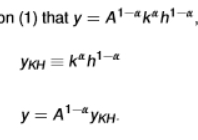
factor-only model

• the first equation is a production function assumption

• we use α = 1/3 as on average across the world and across time, physical capital earns about 1/3 of national income

• when we are measuring success, we are asking: suppose that all countries had the same level of efficiency A, what would the world income distribution look like in that case, compared to the reality?

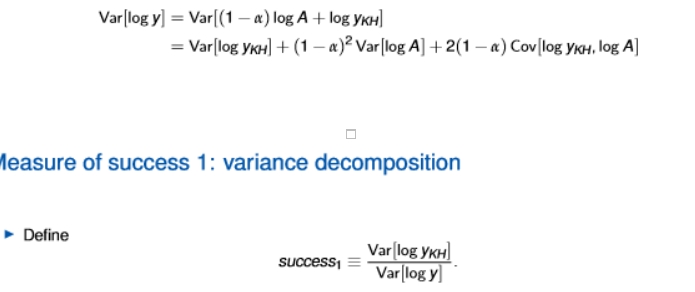
variance decomposition - measure of sucesss of the factor-only model in explaining income differences

• we take the factor-only model in log form

• log y = (1 - α)logA + logy_kh

• the labour share (1-α) is scalar

• the interpretation of the covariance: as the factors go up, how much does TFP go up? (this is significant as they usually grow together)

• we expect the covariance to be large and positive

• the success formula is similar to the r-squared formula

• if A was some constant, all the variation would be explained by the y_KH (factor component)

• this would result in success = 1

• if we have more factors, we would have a higher TFP (we would then assume we are using them more efficiently)

• if A varies across observations, then the var(logA) > 0

• if cov(logy_KH, logA) >/= 0 as well (meaning that observations with more factors tend to have a higher A), then var(logy) >0 so success<1

• very sensitive to outliers

• asks what would the dispersion of (log) per capita income be if all countries had the same level of efficiency, and then compares this counter-factual dispersion to the observed one

variance of linear combination formula

• when x and z are variables, a and b are parameters, the variance of the linear combination ax +bz is what is in the picture

• it depends on the individual variances in the squared scalar form and their covariance

• DON’T FORGET ABOUT THE COVARIANCE EVER!!

interpercentile range - measure of sucesss of the factor-only model in explaining income differences

• we are measuring the 90th to 10th percentile (in terms of y_KH and y)

• we are measuring the distribution of factors vs the distribution of income

• the ratio between the 90th and the 10th percentile of the income distribution is about 21

• less sensitive to outliers

• compares what the 90th-to-10th percentile ratio would be in the counterfactual world with common technology to the actual value

comments about accounting success across countries

• the measure of success using variance decomposition is about 1/3 which means that about 1/3 of GDP per worker across time can be accounted for by factor intensity

• it is a bit higher in China and a bit lower in India

• the measure of success using interpercentile range is around 2/3 (though a bit lower in India), meaning that according to this measure, factors matter more

• combining the two measures of success, we can say that about ½ of the time variation in GDP per worker is explained by physical (investment) and human (years of schooling) capital

• this only applies for the four countries chosen (US, UK, China, India)

comments about accounting success across time

• both measures of success are more aligned, on average a bit higher than 1/3

• in more recent years, the factor-only model’s explanatory power decreases

• one of the reasons may be sample selection; over the years, the sample of countries (in particular poor ones) increases

• a very rough conclusion is that a bit more than 1/3 of the cross-country variation in GDP per worker is accounted for by factors

• much of the GDP variation is still not accounted for - the variation in the ‘unexplained’ component total factor productivity A is large

can we improve the explanatory power of the factor-only model?

• basic adjustments such as depreciation, initial capital, years of schooling, are unlikely to make a large difference

• more important adjustments that may give more explanatory power to the factor-only model (but are also more difficult to implement) are those related to improved equality-based measures of h and k

• better adjustments for quality of capital will probably improve the explanatory power of the factor-only model, but uncertain by how much

quality of schooling as alternative measure of h to better account for quality differences to improve the factor-only model

• before, we were assuming a year of schooling is the exact same in every country when quality actually differs

• this means that our measure of h is exaggerated

• human capital is richer in countries that have higher quality of schooling that in poorer countries (a rich country should not get the same level of human capital from one year of schooling compared to a poor country)

• this can help to explain more of the income differences between rich and poor countries

• as income increases, so does the quality of schooling so we assume the human capital has higher quality in richer countries than in poorer countries

• if we factor this into the model, it will be able to explain more of the variation as we created more variation in human capital across time

experience as alternative measure of h to better account for quality differences to improve the factor-only model

• human capital accumulates through work experience

• in poor countries, workers have, on average, more work experience (as they work longer hours, spend less time in school, and retire later)

• they typically seem to have lower returns from experience (implying that less human capital is accumulated on the job)

• on balance, this effect is therefore not too important

health as alternative measure of h to better account for quality differences to improve the factor-only model

• workers in poorer countries are typically less healthy (eg due to nutrition, exposure to pathogens, lack of medical care), which can impair physical and cognitive function

• this can exaggerate our measure of h

• it is difficult to measure, most reasonable estimates do not suggest large effects

R&D content of physical capital as alternative measure of k to better account for quality differences to improve the factor-only model

• the quality of physical capital k is probably lower in poorer countries because of lower R&D content, but the magnitude of this effect is difficult to establish

what could the large differences in overall efficiency (TFP) found in the aggregate level reflect?

• could reflect large differences in efficiency within each sector of the economy

• could also be due to the fact that some countries have more of their inputs intrinsically less productive sectors than others

• for example, poor countries have as much as 90% of their workforce in agriculture while rich countries have as little as 3%

• only a small fraction of the overall variation in efficiency is due to differences in sectorial decomposition

• efficiency differences appear to be a within industry phenomenon

what countries uses physical and human capital more efficiently?

• poor countries use human capital more efficiently

• rich countries use physical capital more efficiently

return to one extra year of education for different countries

• in sub-saharan Africa (lowest levels of education), the reutn to one extra year of education is about 13.4%

• the world average is about 10%

issues with our measures of success

• success is highest in the Americas, with roughly 50% of the log income variance explained and lowest in Europe with 23%

• the result found in Europe is due to the inclusion of Romania, whose very high level of human capital makes it difficult to explain its very low income

• when Romania is excluded, the success of the factor-only model for Europe is virtually perfect

• this means that the factor-only model works the worst where we need it the most, ie when poor countries are involved

what type of factors are physical capital, labour, and land?

• physical capital is an endogenous production factor (built through investment/saving

• this means it doesn’t appear from nowhere

• labour and land are exogenous

law of motion of capital equation

• capital depreciates at the rate δ e (0,1) (in a range between 0 and 1)

• new capital tomorrow equals the undepreciated capital left of today plus new investment It

• the initial capital K0 > 0 is exogenous

setup for the solow model

• time t is discrete and runs from 0 to infinity

• one single representative agent (representative household and/or representative firm):

• owns all capital and supplies all labour in the economy

• makes all decisions

investment equation for solow model

• only thing that households can do is choose savings

• it invests (saves) an exogenous fraction s between a range of 0 to 1 of income/output Yt

• this variable ‘s’ is important as the higher it is, the more capital that can be accumulated

resource constraint formula in solow model

• anything that is not invested is instead consumed

• Ct = Yt - It

production function for output Y in solow model

• AL = labour-augumented

• A = TFP

• human capital is incorporated into A

• in the simplest version of the solow model, we keep A (TFP) and L (labour/population constant

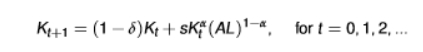
capital law of motion/law of motion of economy equation

• we are combining the production function equation and the savings equation

• we are starting from K0

• once we know this initial capital stock, we can compute the capital stock in every period

• once we know the series of Kt, we also know all the other variables

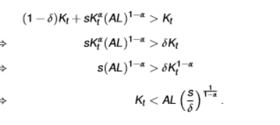
what is the condition for positive capital growth, Kt+1 > Kt in the solow model?

• we use the law of motion of economy equation

• the second equation is saying that capital is growing if we invest more into new capital each period than we are losing capital due to depreciation

• if we start below (K <), then K will grow from t to t+1 (as shown in the picture)

• if we start above (K >), then K will fall from t to t+1

• since production Yt = K(AL) is increasing in capital, Kt+1 > Kt implies Yt+1 > Yt while Kt+1 < Kt implies Yt+1 <Yt

• output must be growing if capital is growing as capital is the only thing that can move

• economies can shrink if their depreciation is higher than their investments