Microeconomics

Opportunity cost

The next best alternative given up when making a decision

Opportunity cost=sacrifice in x/gain in good y

Marginal

Analysis of incremental changes

Marginal analysis

Based on the idea that economic agents seek to maximise or minimise outcomes when making decisions

Rational agents

Respond to changes in costs and benefits when making rational decisions

Barter economy

Trade between agents for goods and services

Specialisation and division of labour

Exchange and redistribution of labour and the factors of production to improve productivity and efficiency

Capitalism

• Private ownership of the factors of production

• Goods and services are exchanged through the price mechanism 

• Firms aim to maximise profits

Pure market economy

• No government intervention 

• Agents are left to the devices of the price mechanism (Adam Smith’s- Invisible hand; price and quantity is efficient from cost and benefit analysis by agents which drives supply and demand

Planned economy

Economic activity is determined by government intervention

• Scarce resources are being allocated efficiently

• Micro- direct intervention in markets via things like specific taxes, quotas, and price ceilings

• Macroeconomic policy- e.g. fiscal policy, monetary policy, supply-side policy

Market failure

A situation where scarce resources aren't being used efficiently

Externality

The cost or benefit on a third party from a transaction that isn't considered by the decision maker

Market power

ability of a single economic agent (or small group of agents) to have a substantial influence on market prices or output  e.g monopoly

Market economy

Allocates resources through price signals created by the forces of supply and demand

Positive statements

Claims that attempt to show how the world is and can be proven or disproven

Normative statement

Claims that attempt to show how the world should be and cannot be proven or disproven

Falsifiability

the possibility of a theory being rejected as a result of new data or observations.

Cause and effect

establishing whether one factor causes another (as opposed to correlation).

Assumptions of basic supply and demand model

• There are many buyers and sellers.  Invisible hand- overall changes in a large group of people will impact the market not just individual consumers

• Each buyer/seller has perfect information (or at least “equal” information)

• Firms produce and sell homogenous goods (i.e. identical products)

• The homogenous goods sell at a uniform price

Factors affecting demand

• The number of consumers

• Consumers’ income levels, how much a good/service takes up their income

• tastes/preferences/trends, changes over time for certain goods and services e.g consumers switching renting movies to buying tv subscriptions

• The prices of other goods; subjective to consumer preference

  • Compliments e.g whiteboards and whiteboard pens are complementary good so if price increases for whiteboard ceteris paribus, then qd for pens may decrease

Factors affecting supply

• The number of sellers; how many firms are supplying the good/services

• The cost of inputs (production costs); aim to keep costs low

• The level of technology; R&D- firms will supply more if the level of technology is high; unlikely to decrease- can only improve

• Laws, rules and regulations: govt regulation e.g sugar tax- carried onto consumers since its an inelastic good PED. 

  • Safety regulations e.g all cars having airbags- extra cost for manufacturers so they may decrease qs

• The existence of and extent of sellers’ outside options; firms having more than one product e.g Virgin media- if one product is more profitable then the firm may redirect their resources to that good/service

PED

=%change in qd/%change in price

PED=1 unit elastic

PES

PES=%change in qs/%change in price

XED

XED=%change in qd in x/%change in price of y

Positive= substitutes

Negative= compliments

Giffen good

A good where an increase in price will increase demand

Standard economic model

Trade offs from consumer decision model

Consumer preferences assumptions

• Completeness- assume that rational consumers can rank their options by their preferences e.g i prefer chocolate bars to apples- complete preference regardless of price

• Non satiation (never being full) or monotonicity (wanting more of a good than less)- If given a choice between Basket C: 5 chocolate bars and 2 apples or Basket D: 4 chocolate bars and 1 apple- rational consumer will choose basket C because there is more in that basket

  • Monotonic preferences- always prefer more than less; if consumer prefers basket D they violate the assumption of monotonicity but are complete with their preference

• Transitivity- with 3 choices logical assumption that ensures consistency 

  • If a consumer prefers x to y and y to z then we assume that they must prefer x to z.

Utility

Measure to quantify satisfaction gained from consumption

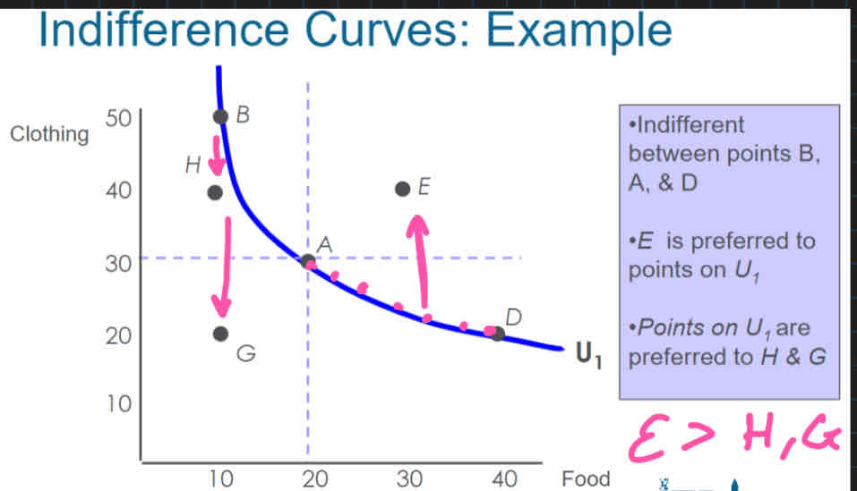
Indifference curve

• Used to represent all combinations or market baskets that a consumer is indifferent between-connects market baskets that give a consumer the same level of satisfaction

• Points below the line- inferior to points on the line; consumer will prefer point/basket on the line than below the line

• Points above the line-superior to points on the line ;consumer will prefer point above to the points on the line

  • Consumers will want the point to be furthest from the origin

• Steep line- prefer what is on x axis, willing to give up more of what's on the y axis

• Shallow line- prefer what is on y axis, willing to give up more of what’s on x axis

  • Straight IC- goods that are readily substitutes for each other

  • Perfect complements are goods for which their utility value relies on them being consumed in fixed proportions with one another.

Diminishing marginal utility

the tendency for the additional satisfaction from consuming extra units of a good to fall.

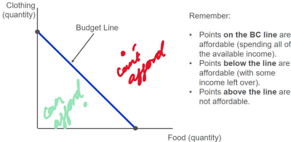
Budget constraints

• Notation of a BC: Y = PfF + PcC maximum of what a consumer can afford; consumers prefer to consume more than less which is why we don’t write Y> PfF + PcC (monotonicity)

• Where; Y = the total income a consumer has to spend, F = the quantity of Food bought, C = the quantity of Clothing bought, Pf = the price of Food, Pc = the price of Clothing

• We assume only 2 goods are consumed

• All the income is spent on the two goods

• Assuming all the prices are constant so the budget constraint is linear

  • The budget constraint line depicts, graphically, all combinations of the two goods that can be afforded with the available income

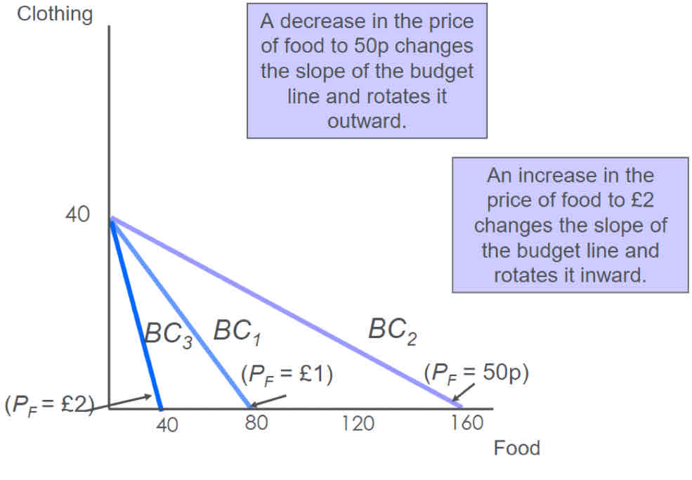
Factors affecting budget constraint line

If one price of a good changes then the slope will change

If the consumers income increases or decreases then there will be a shift

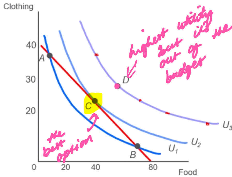
Consumer choice- constrained optimisation problem

Want to maximise utility of the consumption of two goods given the budget

Conditions of utility maximising basket- the optimal choice

• It must be located on the budget line; consumers will want to spend all of their income on the two goods if it is maximising their utility

• It must give the consumer their most preferred combination of goods- point on the budget line that is most preferred; as there are different levels of consumption of each of the two goods on the line- different quantities

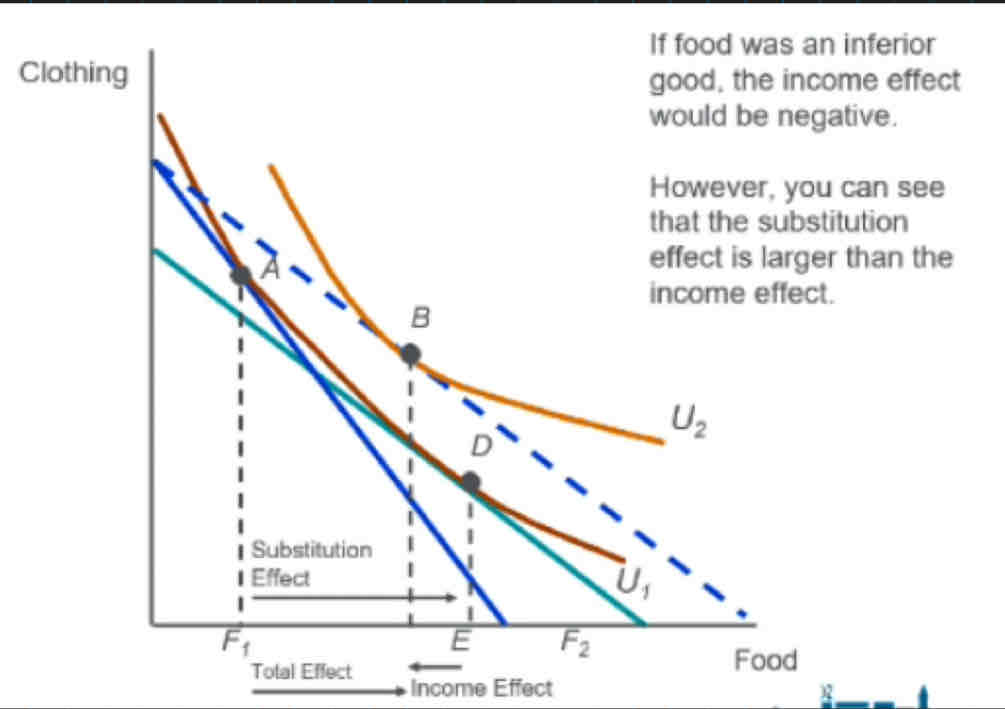
An increase in price of one of the goods (normal)

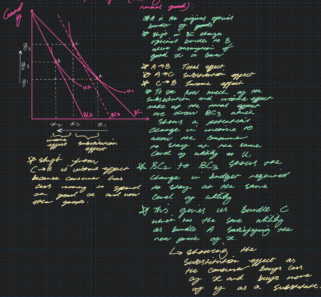
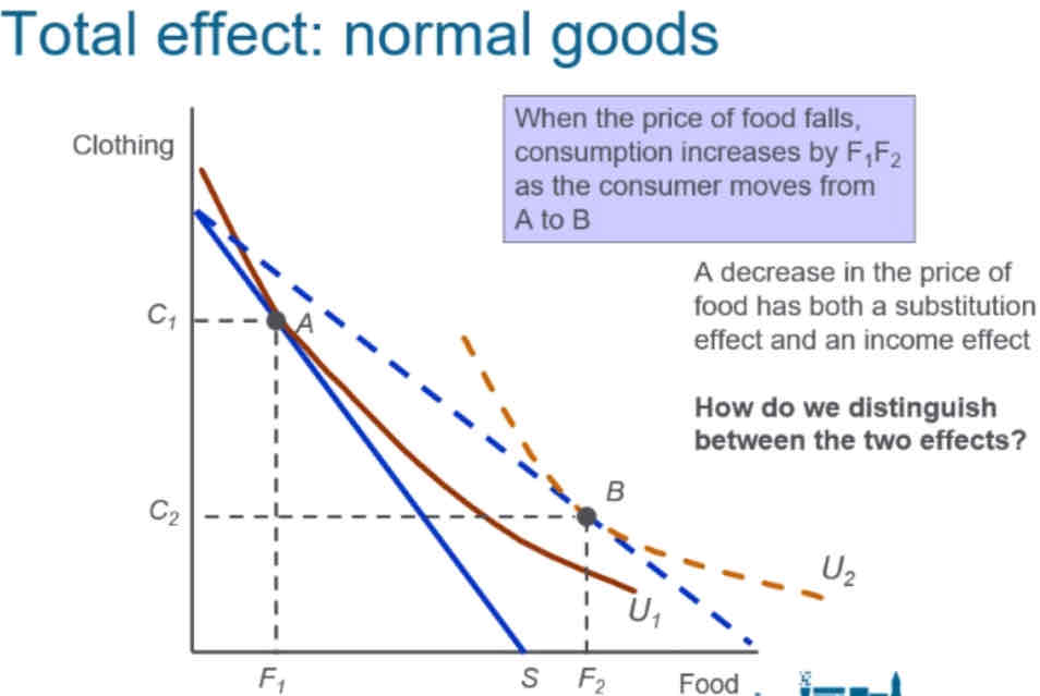
A decrease in price of one good (normal)

Change from point A to point B is the total effect of the decrease in price

• How much of that increase of food demanded is due to the income effect; consumer feels richer and how much of the increase in food demanded is because of the substitution effect 

• Second indifference curve is drawn lower on the budget constraint as there is both a positive income and substitution effect

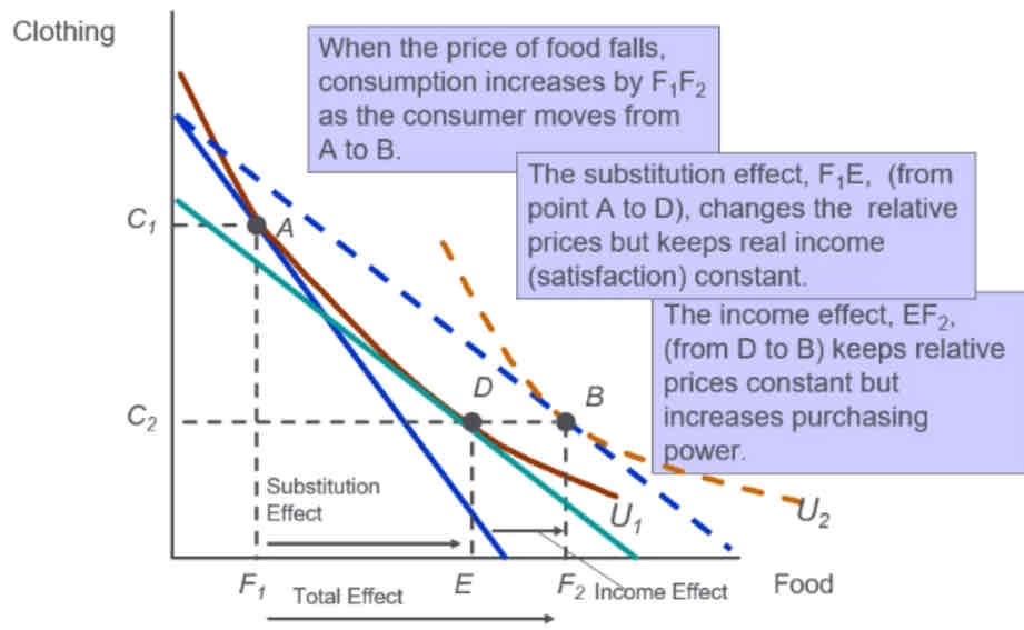
Inferior goods decrease in price

The direction of the substitution effect is always the same – a decrease in the price of a good always leads to an increase in the consumption of that good- always going to switch from th emore expensive thing to the cheaper thing

• However, the income effect can move demand in either direction, depending on whether the good is normal or inferior.

• If a consumer feels like their income has gone up (even though income stays the same) demand less of an inferior good

• Inferior goods have negative income effects; moving to a point where the final point is lower than with substitution effect

  • Inferior goods are ones where as income rises, consumption falls.

  • Hence, inferior goods are ones where the income effect is negative.

• However, note that that the income effect is seldom large enough to outweigh the substitution effect (so as the price of an inferior good falls, its consumption almost always increases)

 

Explicit costs

costs for a firm that requires a direct outlay (an amount of money spent on something) of money such as rent that a firm may need to pay for the building that they are selling their goods/services from

Implicit costs

costs a firm pays without any outlay of money such as earning money if the firm produced a different item than the one they were currently producing (which would be an opportunity costs)

Normal profit

• Normal profit- money to make production happen, beyond this is supernormal profit which can be reinvested e.g to become more dynamic efficient in the LR

Costs as an opportunity costs

if a firm invests into capital instead of saving their money and accumulating interest on their savings an opportunity cost may be the interest that the firm could have otherwise received

Short run costs

some costs are fixed e.g size of a factory is fixed but the number of workers is variable can increase more workers to increase output -can lead to overcrowding and poorer quality output diminishing marginal product

Long run costs

fixed costs become variable costs- how long is the long run

Diminishing marginal product

where the marginal product of an input decreases as the quantity of the input increases e.g more workers in a factory using the same amount of machinery may lead to overcrowding due to limited amount of equipment

• Eventually diminishes towards 0 as more resources are inputted 

• Only works in SR 

Fixed costs

not determined by the amount of output     produced; they can change but not as a result of changes in the amount produced e.g rent which needs to be paid regardless of how much a firm is producing or machine- wouldn’t be able to make changes easily on rent and expensive machinery in the SR

Variable costs

change as the firm alters the quantity of output produced e.g water or electricity bills which are based on per unit or employees which can be changed quickly -however dependent on labour laws for hiring + firing employees i.e unions and qualifications for certain skilled occupations

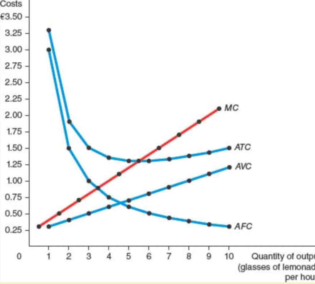
shapes of cost curves

ATC is a U shape-

• AFC always declines as output rises because the FC does not change as output rises and so gets spread over a larger number of units

• ATC declines as output increases- The bottom of the ATC curve (where MC intercepts) occurs at the quantity that minimises average total cost. This quantity is sometimes called the efficient scale of the firm- the quantity that minimises ATC

• ATC starts rising because AVC kick in and rise substantially as more units are being produced with the same fixed costs e.g lower productivity when there's overcrowding

• MC and ATC:

  • When MC<ATC, ATC is falling -down the u-shape

  • When MC>ATC, ATC is rising -up the u shape

  • The MC=ATC at the minimum efficient scale- minimum efficient scale is the quantity that minimises average total cost

  • MC is upwards sloping because of the property of diminishing marginal product to the variable input

Long run and short run average costs

The LRATC curve lies along the level of output that is optimal/low/lowest points  of the SRATC curves because the firm has more flexibility in the long run to deal with changes in production:

• The length of time for  firm to get to the LR will depend on the firm involved e.g pharmaceutical firm vs restaurant

• SR- some f.o.p cannot be changes

• LR all f.o.p/factor inputs can be changed e.g can build more factories or can liquidate assets 

  • Sunk costs shouldnt be considered in the SR

• Goals in SR and LR are the same when the SRATC is the same as the LRATC i.e where they intercept e.g firm may want 1 factory in the SR but that also may be their goal in the LR too

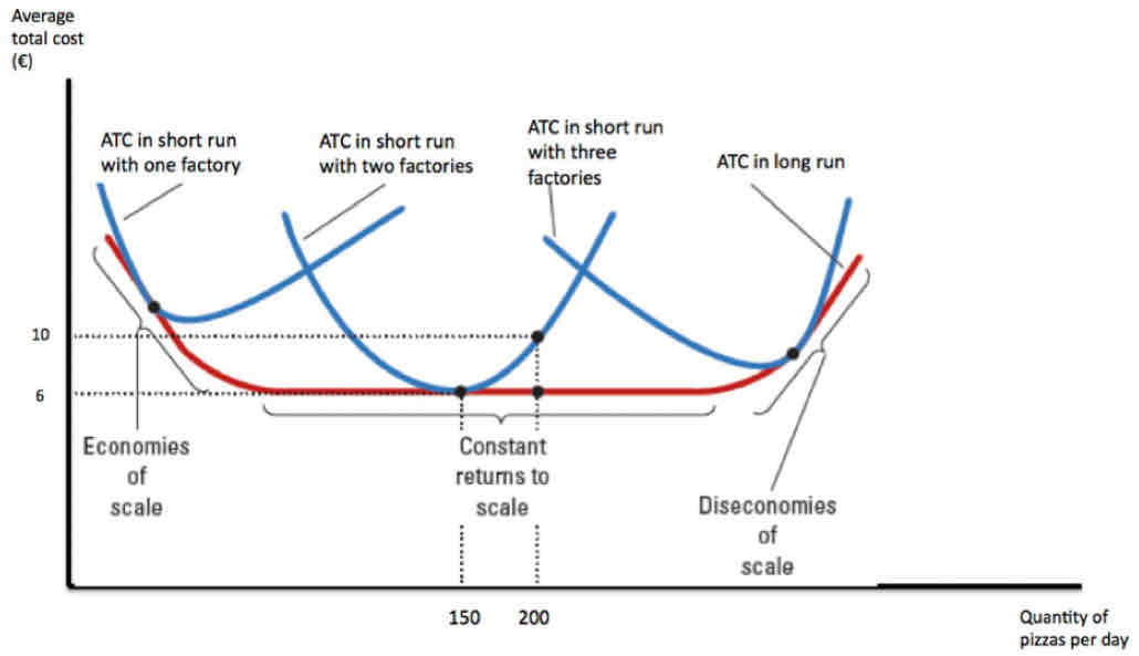
Economics of scale

• Constant returns to scale the property whereby long-run average total cost stays the same as the quantity of output change

• Economies of scale the property whereby long-run average total cost falls as the quantity of output increases.

• Diseconomies of scale the property whereby long-run average total cost rises as the quantity of output increases

Commercial economies of scale/ bulk buying

• E.g. negotiate lower prices for factor inputs

Financial economies of scale- instability, how wise is this in the LR

• Larger firms can borrow at lower costs and can also issue bonds.

Managerial economies of scale

• Large firms employ specialist managers- may lead to mismanagement

Risk bearing economies of scale

• Large firms can diversify and invest more in R&D e.g  can invest in different types of goods/services like Virgin; silicon valley?

External economies of scale

from locating where there is a specialist pool of labour or the infrastructure is better:

• the advantages of large- scale production that arise through the growth and concentration of the industry

Diseconomies of scale

arise due to coordination and communication problems that are occur in a large firm

• X-inefficiency- the failure of a firm to operate at maximum efficiency due to a lack of competitive pressure and reduced incentives to control costs e.g monopoly firm may have x-inefficiency

Assumptions of a perfectly competitive market

• There are many buyers and sellers in the market- the actions of any single buyer or seller in the market have a negligible impact on the market price; must accept price determined by the market; concentrations in market structures e.g monopolies (which determine the market price) or oligopolies (can collude to determine a market price)

• The goods offered by the various sellers are largely the same- homogeneous goods; quality and properties of the goods are the same- no product differentiation/USPs

• Firms are price takers- Buyers and sellers must accept the price determined by the market since they don’t have the power to set their own prices

• Firms can freely enter or exit the market- no exit or entry costs; for example- if everyone is making a loss then the market may shrink; e.g decrease in supply/firms leaving the market to make price reach the new equilibrium point

Perfectly competitive revenue

• Total revenue for a firm is the selling price times the quantity sold

• TR = (PxQ), P is fixed (price takers) so Q is the only thing a firm can change

• Total revenue is proportional to the amount of output

• TR=PxQ and AR=TR/Q which means that in a perfectly competitive market AR=P

  • Rearrange TR=PxQ to be P=TR/Q so P=AR

• MR=change in revenue/change in quantity=AR curve, change in revenue/change in quantity is the same amount at each level of output so MR stays the same so MR=AR=P

Normal profit

the minimum amount required to keep factors of production in their current use

Abnormal profit

Profit above normal profit

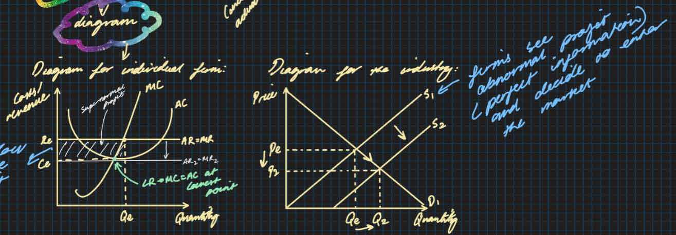
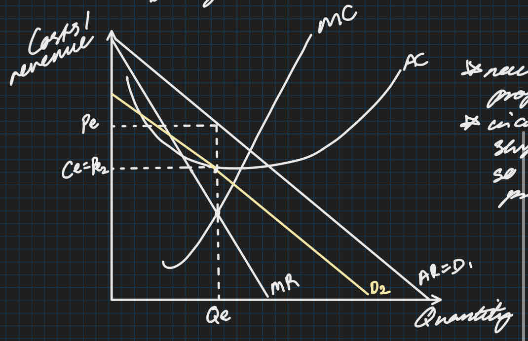
Perfectly competitive long run changes diagram

Isoquants and isocosts

A production isoquant (iso=equal, quant=quantity) is a function which represents all the possible combinations of factor inputs that can be used to produce a given level of output

• Costs when introducing new levels of output which require levels of inputs; so isoquants help work out what the best level of input is at the optimal level

Using the f.o.ps:

Firms choose different ratios of factor inputs, land, labour and capital, in the production process- 

• Highly labour intensive – high ratio of labour to other factors

• Highly capital intensive –high ratio of capital to other factors

• Highly land intensive- high ratio of land to other factors

  • Organising the factors of production to maximise output at a minimum cost

  • Trading off one factor for another leading to different ratios

• The use of isocost and isoquant lines provides a model to help illustrate the process

  • Optimal level of output through finding the best combination of f.o.ps with the lowest cost

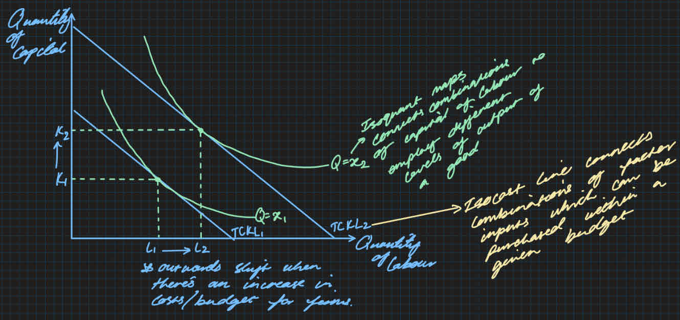
Slope of isoquant line- marginal rate of technical substitution MRTS

This is the rate at which one factor input can be substituted for another at a given level of output

MRTS=MPK/MPL 

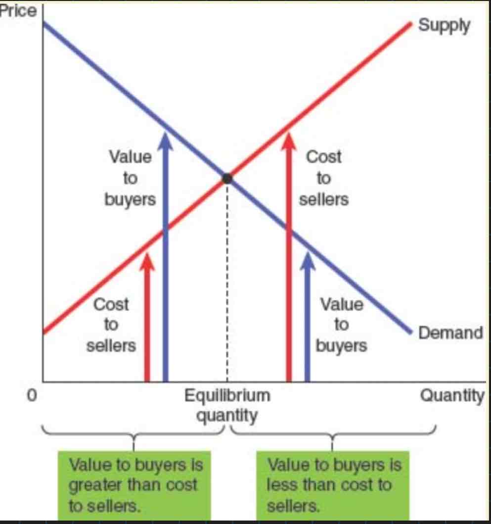
Allocative efficiency

• occurs when the value of the output that firms produce (the benefits to sellers) matches the value placed on that output by consumers (the benefit to buyers)

  • Buyers and sellers receive benefits from taking part in the market

  • The equilibrium in a market maximises the total welfare of buyers and sellers

  • This analysis is based on the assumptions that consumers have monotonic preferences (more consumption leads to more utility- diminishing marginal utility) and can rank their preferences

Objective well-being

refers to measures of the quality of life and uses  indicators developed by researchers e.g educational attainment, measures of the standard of living and life expectancy.

Subjective well being

refers to the way in which people evaluate their own happiness e.g how people feel about work and leisure.

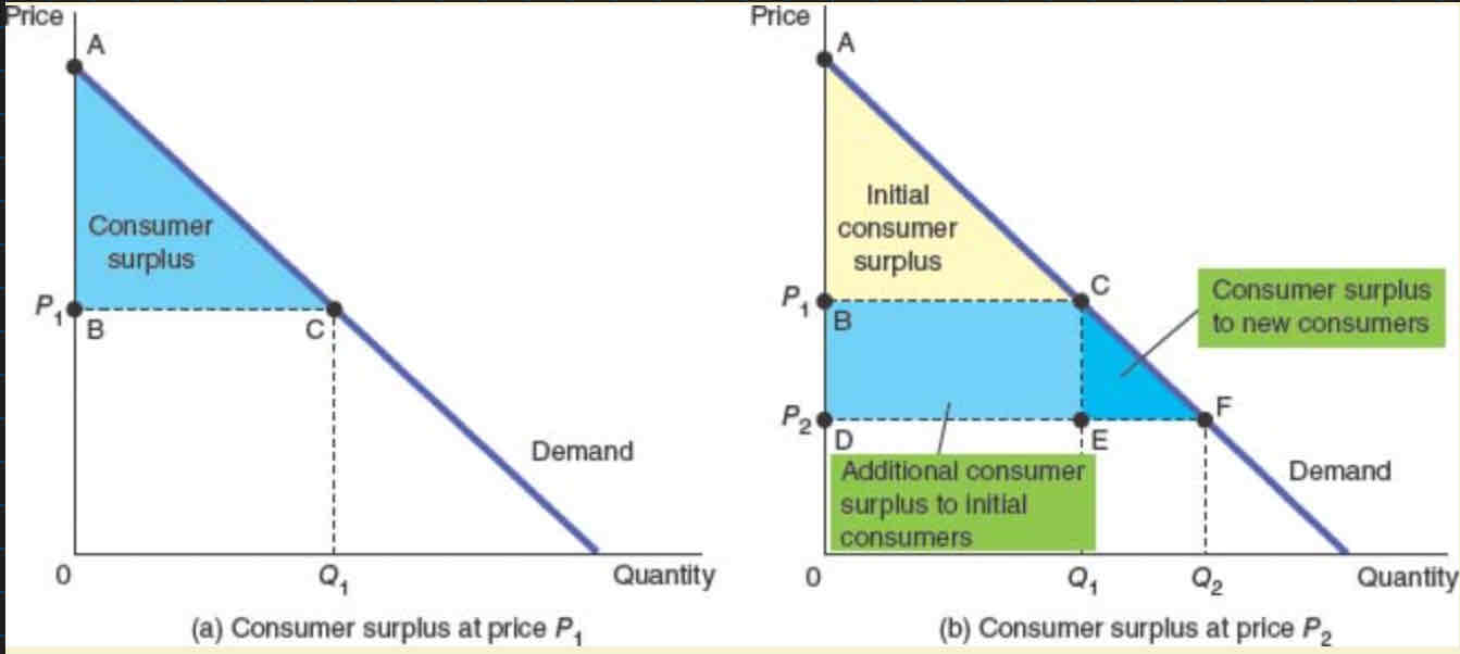
Consumer surplus

buyer’s willingness to pay minus the amount the buyer actually pays for it

• Willingness to pay- maximum amount that a buyer will pay for a good; it measures how much the buyer values the good or service e.g consumer may value a guitar at a £300 and that would be the maximum amount that they would pay

• Bargain paying much less for something than we expected or anticipated leading to a greater degree of a consumer surplus

• measures the benefit that buyers receive from a good as the buyers themselves perceive it

Bargaining process

an interaction resulting in an agreed outcome between two interested and competing economic agents 

• Suppliers are offering goods to consumers at different prices, and consumers must make decisions about whether the prices offered represent a net economic benefit to them

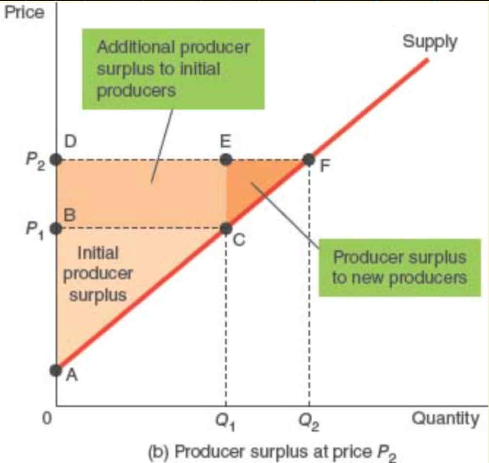
Producer surplus

Producers would be eager to sell their services at a price>costs, would refuse to sell their services at a price<costs, and would be indifferent about selling their services at a price=cost

• Cost is the value of everything a seller must give up to produce a good

• Producer surplus=amount a seller is paid for a good - cost

• It measures the benefit to sellers participating in a market

Keynesian labour markets

• Hard for markets to clear if there are barriers to change wages; sticky prices (don't change instantly to market forces) in the SR- workers prefer certainty over varying pay e.g offering lower wage with guarantee that it'll stay the same (fixed wages)

• Reluctant to change wages if employees leave- altered firm behaviour 

• Menu costs; extra costs of changing menus- in advance so if costs of production increases firms may be stuck with their current prices if they are stuck in a contract when they want to cover their costs with higher prices- incentives to alter behaviour but constraints preventing them to do so which make it difficult to adjust behaviour- speed of markets moving to equilibrium may be very different depending on negotiated arrangements for example, can’t liquidate assets immediately if you want to cover costs

Pareto improvement

occurs when an action makes at least one economic agent better off without harming another economic agent- helps reduce waste in an economy e.g in monopoly where there is a deadweight loss when the loss could be diminished; difficult for this to occur?- when there isn't pareto efficiency

• Consumers and producers will continue to readjust their decision-making with the resulting reallocation of resources until there are no further Pareto improvements. We can view economic efficiency in terms of the point where all possible Pareto improvements have been exhausted

Pareto efficiency

occurs if it is not possible to reallocate resources in such a way as to make one person better off without making anyone else worse off

• E.g in production potential frontier- no way to make one person better off without making the other worse off; one person has 0 of x, and another has 100- to reallocate resources the other person will lose some of their good x

• Where all opportunities of pareto improvement are not there when the equilibrium is pareto efficient- competitive equilibria are pareto efficient

Market effficiency and the social planner

Left of equilibrium- incentive to buy more and for sellers to sell more

Right of equilibrium- incentive for buyers to buy less and for sellers to sell less

Competitive equilibrium is an efficient allocation of resources agents have responded to prices and prices have responded to prices 

Efficiency is a positive concept as it can be defined and quantified (all resources being employed with minimal waste):

• The social planner's problem is to maximise consumer welfare given the technology and the resource constraints. Thus, the Pareto optimum is the allocation that a social planner would choose

  • Because the equilibrium outcome is an efficient allocation of resources, the social planner can leave the market outcome how they found it

  • Efficiency vs equity…

Monopolistic competition

Large number of small firms, but those firms have power to change their prices; with product differentiation (non-homogeneous goods) e.g restaurant industry, gaming industry

Product differentiation

• A firm won’t immediately lose all their sales by setting a price above their rivals

• Some consumers prefer Firm A’s product, others prefer Firm B’s product, and for some it might depend on the prices

Assumptions of monopolistic competition

Assumptions of a monopolistic competition:

• Large number of (“small and insignificant”) firms

• Product differentiation *only assumption different to perfect competition

• Free entry and exit (i.e. no barriers to entry)- always barriers e.g incumbent firm advantage

• Complete information- incumbent firms would have more knowledge since they’ve been in the market for longer

 

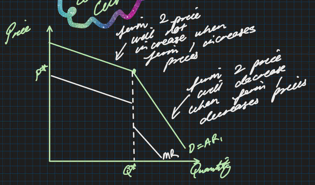
Monopolistic competition diagram

• In SR they behave similarly to a monopoly, same downwards sloping demand curve

• MR is twice as steep as AR/D

• Due to product differentiation the monopolistically competitive firm faces downward-sloping demand (unlike perfectly competitive firms, who face horizontal demand)

• Profit-maximising so choose to produce where MC=MR

• At that optimising point, in the SR, the firm has:

  • Supernormal profit where P>AC

  • Loss if P<TC

• new firms enter the market due to the profit that is available

• If profits were made in the SR, then in the LR more firms will enter the industry

• Those new firms will have a slightly differentiated product, but some consumers will switch their consumption so the demand curves (AR) of incumbent firms will shift to the left

• If losses were made in the SR, then in the long run some firms will exit the industry

• The demand curves of remaining firms will shift to the right

• Always the long run point regardless of whether SR was a loss or profit

• The demand curve (AR) will shift to the point at which P=AC and only normal profit is made – i.e. there will be entry (or exit) until we reach this point

Regulation and advertisement

Regulation- To enforce marginal cost pricing, policymakers would need to regulate all firms that produce differentiated products. Because such products are so common in the economy, the administrative burden of such regulation would be overwhelming + expensive

When firms sell differentiated products and charge prices that are above (marginal) cost, each firm has an incentive to advertise or develop brands to attract more buyers:

Pros of advertising	Cons of advertising
• Advertising provides information to consumers, for example regarding the prices of the goods on sale. • If consumers (and rivals) have more complete information, this is pro- competitive	• Consumers’ tastes may be manipulated – do adverts convey information about product quality? Sometimes yes, sometimes no. • The extent of differentiation may be exaggerated (misinformation); including other goods in an advert e.g for mascara the model may wear a full face of makeup

Oligopoly

very concentrated market, where a small number of firms account for a high portion of sales.

Strategic interdependence

where the outcome for one party depends not only on their own actions but also the actions of others (& the best course of action may depend on what they expect others to do)- making decisions by predicting another party’s behaviour

Strategic behaviour

Since there are so few firms they must pay attention to one another’s decisions. Can make profits in the long run since there are high barriers to entry and they have a high market share.

Kinked demand curve

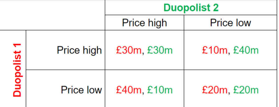
Oligopoly game theory assumptions

• The market is a duopoly (just two firms)

• The firms sell a differentiated product

• The decision variable is price (i.e. firms choose prices and then the quantity they sell is determined by the demand they face)

• Just competing once and never again

Nash equilibrium/mutual best response

Where no player can make themselves even more better off

Private goods

Excludable (can’t consume unless you pay for it) and rivalrous (one persons consumption will stop another persons consumption)

Public goods

Non excludable and non rivalrous

Free rider problem from public goods

A person can enjoy the benefits of consuming a good without paying for it

Merit goods

goods or services that are considered to be beneficial to individuals and society as a whole, but are often under-consumed in a free market economy e.g. education and healthcare which may be state provided as a result

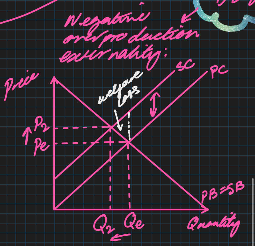
Externalities

Arise when social costs and benefits are not considered in the transaction of goods and services

Social costs

Social costs=external costs + private costs

External- costs to a third party outside of the transaction

Private- costs to the individual in the transaction e.g. price of the good being bought or produced

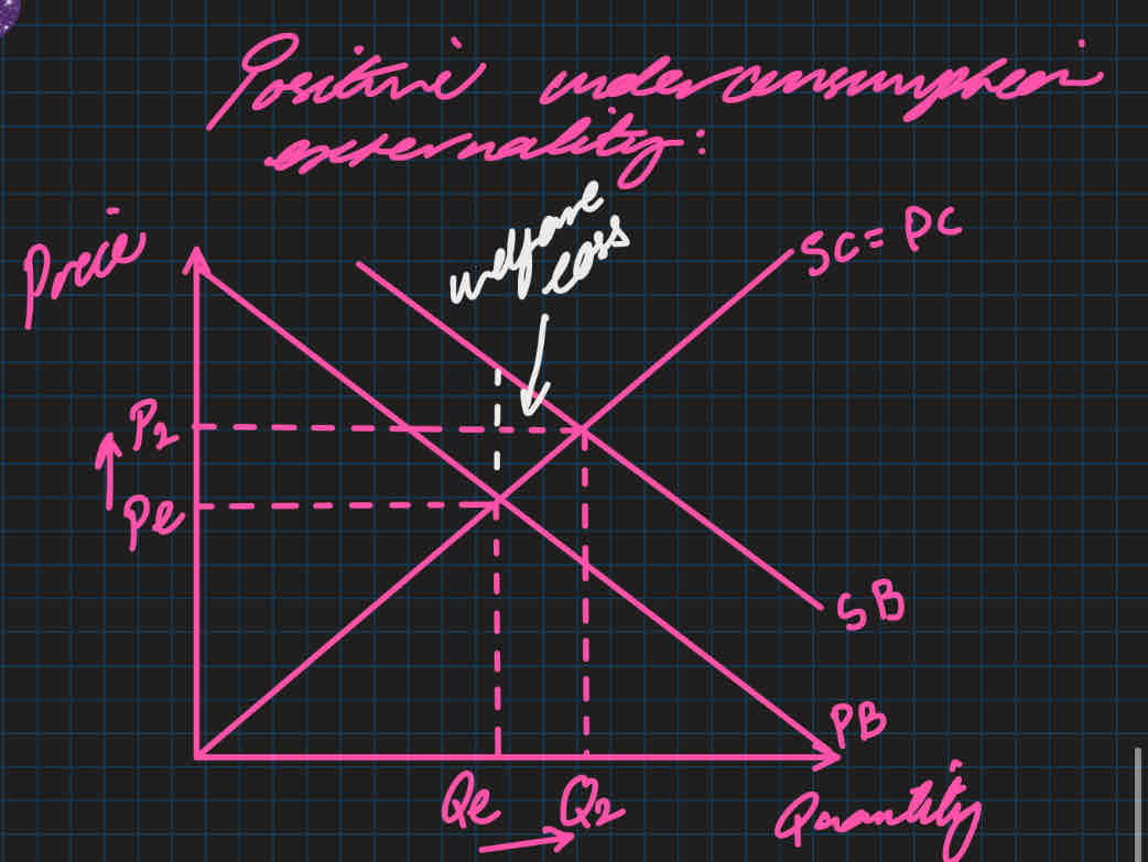
Positive consumption externality

Difficult to actually quantify the social costs and benefits

Coarse theorem

Private parties can bargain with each other to solve externalities

• depends on if there’s symmetrical information

• Depends if both parties have the ability to negotiate

Negative overproduction externality

Solutions to correct externalities

direct taxes- on the price of goods

Ad Valorem tax- %

• difficult to measure how much of a tax is needed

Subsidies for positive externalities

Nationalisation- under govt ownership and control

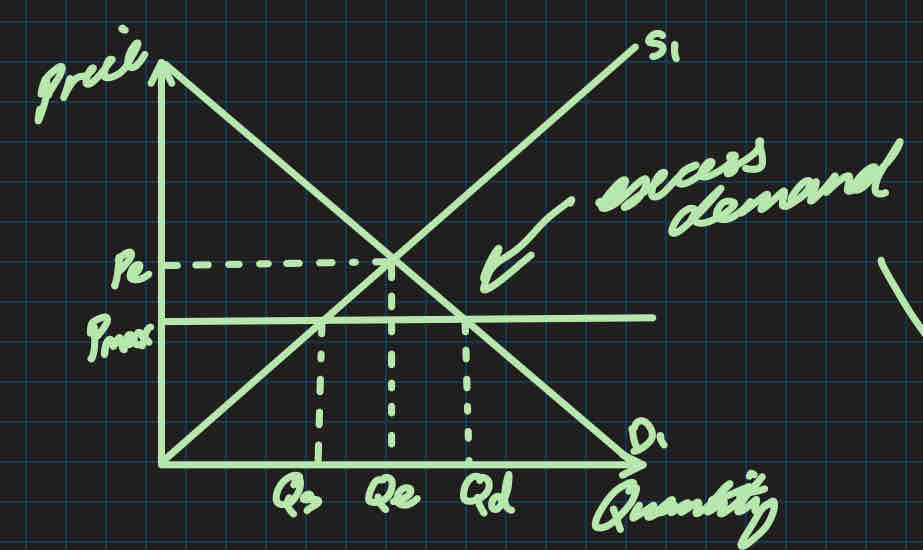
Maximum price

A legal maximum price of a good placed below the price equilibrium

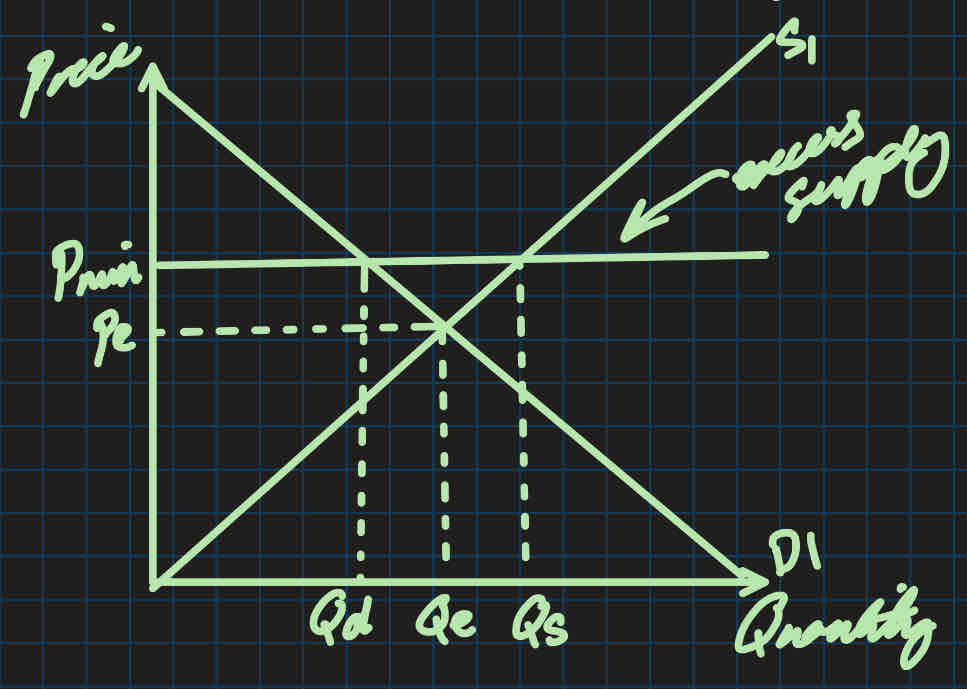
Minimum price

A legal minimum price of a good placed above the price equilibrium

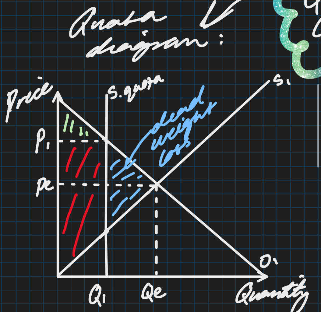
Quantity control quota

• Binding policy so there’s an effect on the market equilibrium

• restricted supply curve so it’s vertical at the set quantity

• Firms will sell max. quantity at new price p1

• Bad intervention because theres inefficiency from the welfare lost

• Good intervention because there’s an increase in surplus but this depends on the function of s and d and PES and PED