part 2

elements of habitat

resources

• food

• cover (including reproductive sites)

• water

environmental conditions

• abiotic

• predators

• competitors

= vegetation, abiotics, other animals

“components” of vegetation

• species composition (= floristics)

• vegetation structure (= physiognomy)

• biomass

• temporal changes in any/all of the above

veg sampling questions to answer

a. What variables will allow you to quantify important “vegetation components”?

b. What spatial scale is relevant to your animal?

c. How should the data be measured & analyzed?

frequency =

percentage of sample units in which a plant species occurs

frequency components

• easy

• good for floristic component

• clumped plant distributions can skew data

• plot size is critical

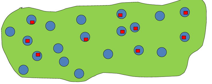
frequency ?

= 10/20 plots = 50%

density =

total number of items (individual plants, stems etc.) per unit area

density components

• labor intensive

• good for physiognomy

• coupled with frequency, height, and cover provides excellent measures of veg

cover =

vertical projection of the crown or stem of a plant onto the ground surface

cover components

• useful indicator of relative dominance, often expressed as %

• crown cover useful for describing forest physiognomy (canopy cover) and grassland forage (grass cover)

• stem cover useful for estimating timber (basal area)

height =

from ground to top of plant

height components

• easy

• sheds some light on physiognomy component but most useful when combined with other measures

tree height =

(% angle to top - % angle to bottom) * baseline distance

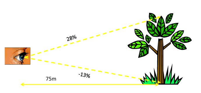
tree height = (28%-- 13%)*75 m = 41%*75= 30.75m

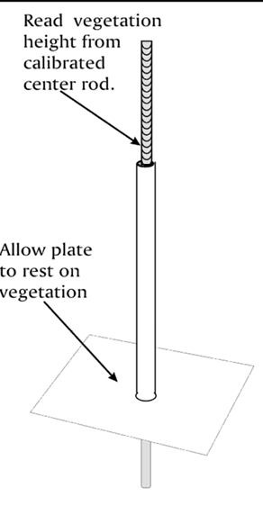
sward stick

• for measuring grassland “height/cover/density”

• plate of known & reported weight (Styrofoam)

plot vs plotless sampling pro/con

• choice of plot size & shape dependent on plant distribution

• usually less precise but also less time consuming

plot sampling

• count # plant spp

• know size of plot

• calculate # indiv./plot = density

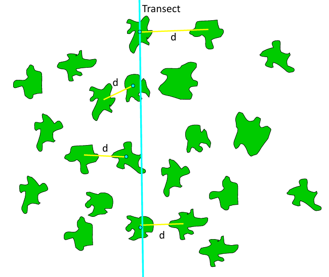
plotless sampling

• dense = small distance between neighbors and/or random points

• sparse = large distances neighbors and/or random points

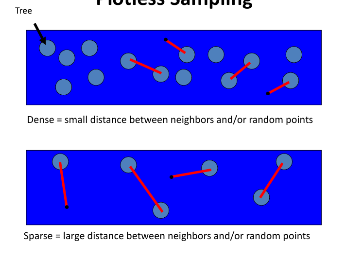
point center quarter method

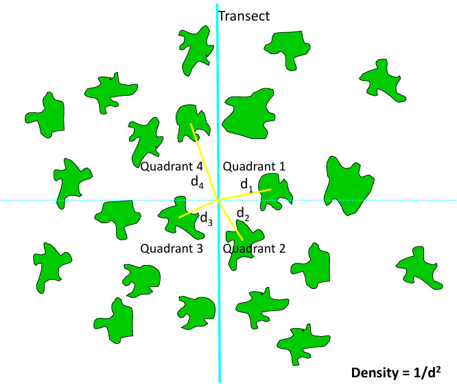
nearest neighbor method

techniques for measuring cover

• quadrat charting

• ocular estimates

• line intercept

• point intercept

• bitterlich variable radius

ocular estimates

• grassland - frames e.g., Daubenmire

• canopy - densiometer

• easy, subject to observe bias

line intercept

• can be used in grasslands, shrublands, or forests

• very commonly used

• quite accurate, somewhat tedious

point intercept

• presence / absence at numerous points

• presence in frames (grasslands) & sighting tubes

bitterlich variable radius

• stem cover in forests or shrublands

• eg cruz-all

• relascope / bitterlich angle gauge

• good for forests w many trees

• no need to measure a fixed plot

• weighting by tree size give ecologically meaningful estimates

biomass =

dry weight of plants in community

biomass components

• useful indicator of food availability for herbivores

• usually expressed as mass per unit area

techniques for measuring biomass

• clipping

• direct estimation

• dimension analysis

clipping

• clip dry and weigh veg

• clip within various “frames”

direct estimation

• for experienced range biologists

• calibration with clipping

dimension analysis

• estimate volume of tree/shrub

• convert to biomass with average density value

miscellaneous vegetation measures

• visual obscurity

• trunk measures

• tree age - rings

• fruits

visual obscurity

• importance to wldf for nesting cover and thermal cover

• weight “density board”

• robel pole

trunk measures

• DBH - 4.5 ft (1.37m) on uphill side (varies)

• basal area - trunk cross-sectional area

fruits (hard and soft mast)

• traps

• transect counts of fallen mast

• visual counts of suspended mast