graph explanations microeconomics

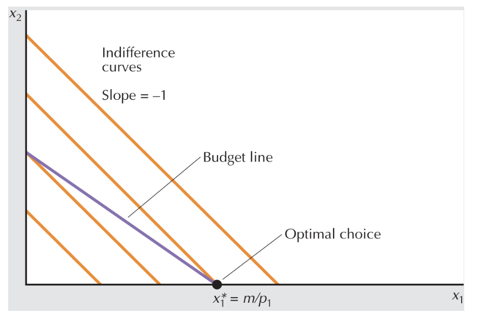
perfect substitutes budget line and IC’s

We have three possible cases. If p2>p1, then the slope of the budget line is flatter than the slope of the indifference curves. In this case, the optimal bundle is where the consumer spends all of their money on good 1. If p1>p2, then the consumer purchases only good 2. Finally, if p1=p2, there is a whole range of optimal choices—any amount of goods 1 and 2 that satisfies the budget constraint is optimal in this case. so basically

optimal quantity of x1=m/p1 when p1<p2

= any number between 0 and m/p1 when p1=p2,

and =0 when p1>p2

All they say is that if two goods are perfect substitutes, then a consumer will purchase the cheaper one. If both goods have the same price, then the consumer doesn’t care which one they purchase.

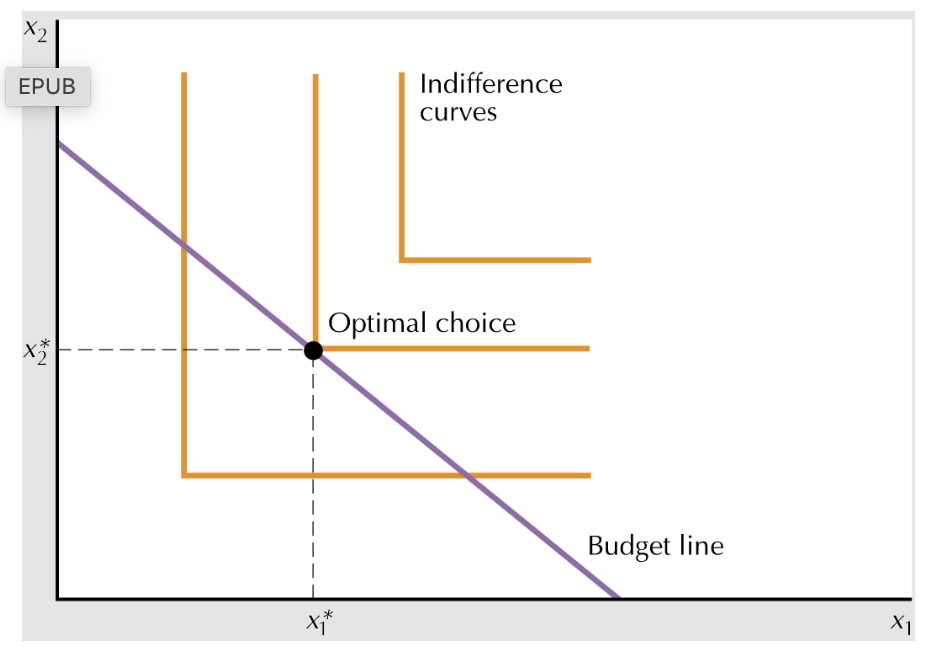
perfect complements budget line and IC

the optimal choice must always lie on the diagonal, where the consumer is purchasing equal amounts of both goods, no matter what the prices are. In terms of our example, this says that people with two feet buy shoes in pairs.2

x1=x2=x=m/(p1+p2).The demand function for the optimal choice here is quite intuitive. Since the two goods are always consumed together, it is just as if the consumer were spending all of their money on a single good that had a price of p1+p2.

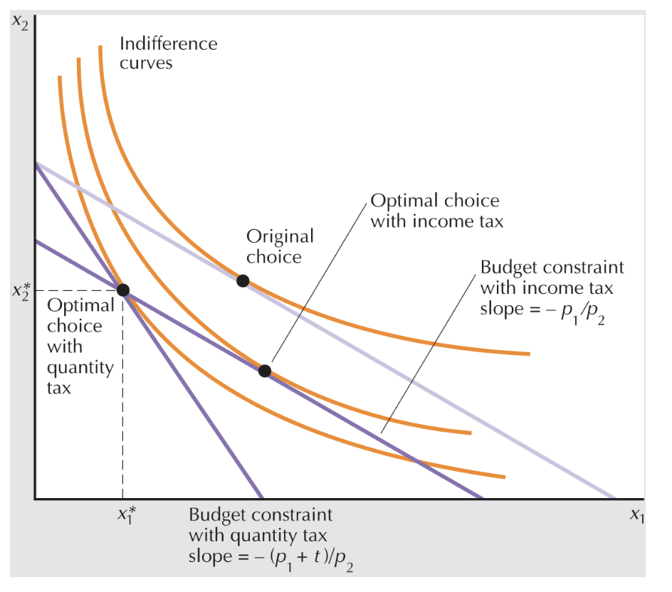
income tax vs quantity tax on budget constraint

original budget constraint p1×1+p2×2=m. if we tax good x1 at rate t, we now have budget constraint: (p1+t)x1+p2×2=m, so the tax revenue is tx1

Let’s now consider an income tax that raises the same amount of revenue. The form of this budget constraint would be p1⁢x1+p2⁢x2=m−R∗or, substituting for R∗, p1×1+p2×2=m-tx1.

it should still pass through x1*,x2*, so we see an income tax is better than quantity tax.

note: a uniform income tax for all consumers is not necessarily better than a uniform quantity tax for all consumers. (Think about a case where some consumer doesn’t consume any of good 1—this person would certainly prefer the quantity tax to a uniform income tax.)

we have assumed that when we impose the tax on income the consumer’s income doesn’t change. We have assumed that the income tax is basically a lump sum tax—one that just changes the amount of money a consumer has to spend but doesn’t affect any choices they have to make. This is an unlikely assumption. If income is earned by the consumer, we might expect that taxing it will discourage earning income, so that after-tax income might fall by even more than the amount taken by the tax

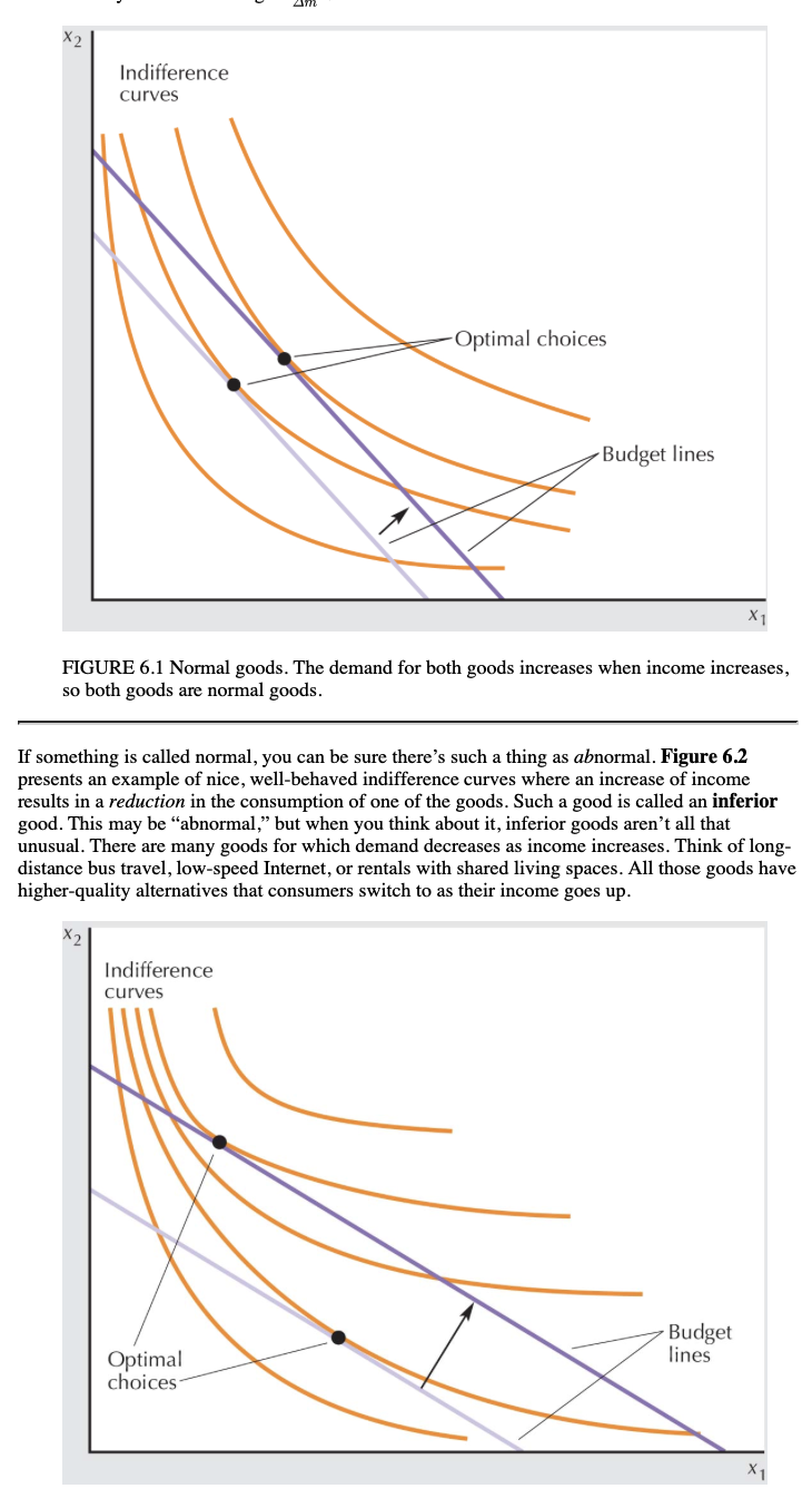
normal and inferior goods on budget lines

• first panel both are normal goods, as budget line moves outward, ie m increases, both goods are consumed more of

• pasnel 2, good 1 is an inferior good, as m increases, budget line moves outwards, but x1 consumption declines and more of x2 is consumed

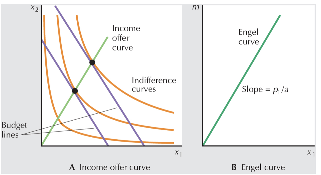
income offer/engel curve with Cobb Douglas preferences

engel curve on right shows relation between income and consumption of good 1.

For the case of Cobb-Douglas preferences it is easier to look at the algebraic form of the demand functions to see what the graphs will look like. If u⁡(x1,x2)=x1^ax2^a-1, where a is fraction of income spent on good x1. the Cobb-Douglas demand for good 1 has the form x1=am/p1. For a fixed value of p1, this is a linear function of m. Thus doubling m will double demand, tripling m will triple demand, and so on. In fact, multiplying m by any positive number t will just multiply demand by the same amount.

homothetic preferences ICs and engel curve

Suppose that the consumer’s preferences only depend on the ratio of good 1 to good 2. This means that if the consumer prefers (x1,x2) to (y1,y2), then they automatically prefer (2x1,2x2) to (2y1,2y2), (3x1,3x2) to (3y1,3y2), and so on, since the ratio of good 1 to good 2 is the same for all of these bundles. In fact, the consumer prefers (tx1,tx2) to (ty1,ty2) for any positive value of t. Preferences that have this property are known as homothetic preferences. It is not hard to show that the three examples of preferences given above—perfect substitutes, perfect complements, and Cobb-Douglas—are all homothetic preferences.

If the consumer has homothetic preferences, then the income offer curves are all straight lines through the origin, as shown . More specifically, if preferences are homothetic, it means that when income is scaled up or down by any amount t>0, the demanded bundle scales up or down by the same amount. This can be established rigorously, but it is fairly clear from looking at the picture. If the indifference curve is tangent to the budget line at (x1∗,x2∗), then the indifference curve through (tx1∗,tx2∗) is tangent to the budget line that has t times as much income and the same prices. This implies that the Engel curves are straight lines as well. If you double income, you just double the demand for each good.

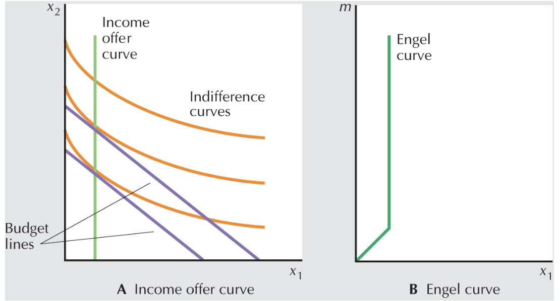
quasi linear preferences, ICs, and engel curves

the utility function for these preferences takes the form u⁡(x1,x2)=v⁡(x1)+x2 What happens if we shift the budget line outward? In this case, if an indifference curve is tangent to the budget line at a bundle (x1∗,x2∗), then another indifference curve must also be tangent at (x1∗,x2∗+k) for any constant k. Increasing income doesn’t change the demand for good 1 at all, and all the extra income goes entirely to the consumption of good 2. If preferences are quasilinear, we sometimes say that there is a “zero income effect” for good 1. Thus the Engel curve for good 1 is a vertical line—as you change income, the demand for good 1 remains constant.

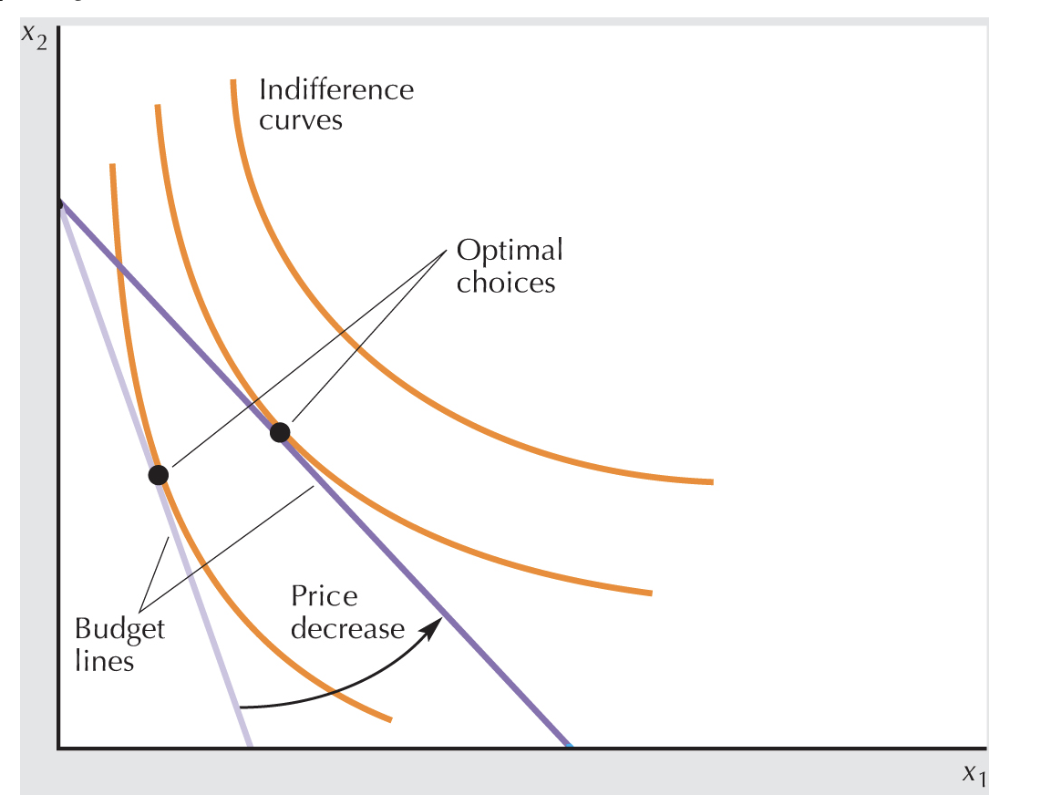
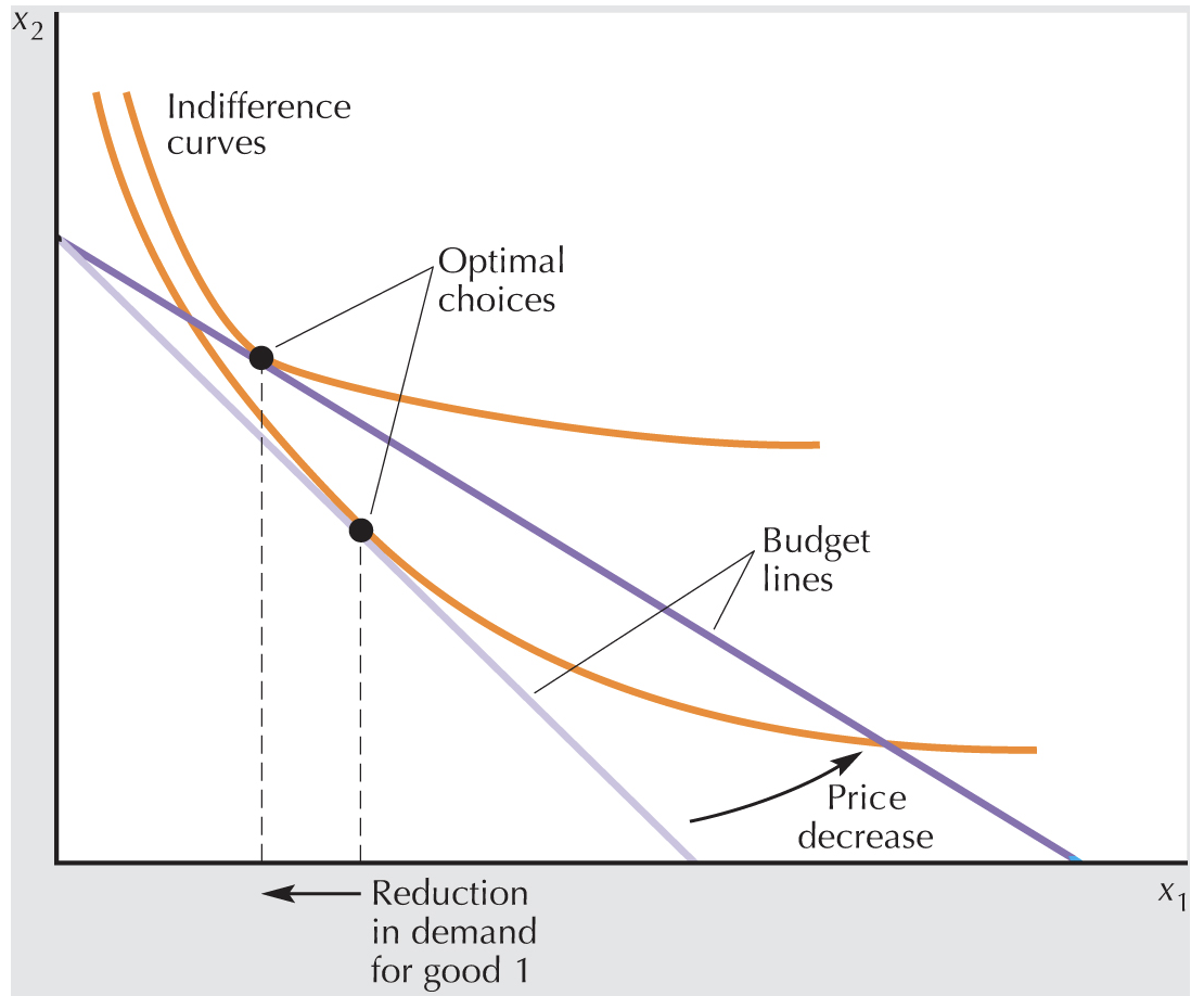
ordinary good price drop on budget lines

Ordinarily, the demand for a good increases when its price decreases, as is the case here.

Giffen good on budget lines, where price of good 1 decreases

The decrease in the price of bread has the same effect as an increase in income: it increases households’ purchasing power. But poor households use that increased purchasing power to lower their bread consumption, instead of raising it. Recall that inferior goods are characterized by this type of negative relationship between income and demand. We will return to the connection between Giffen goods and inferior goods in a later chapter.

Although Giffen goods are perfectly plausible in principle, in the real world they are relatively rare. Most goods are ordinary goods, whose demand declines when the price increases. We’ll see a little later why this is the usual situation.

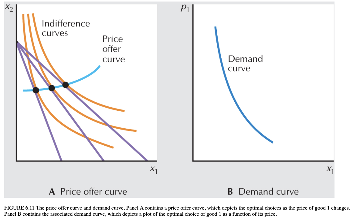
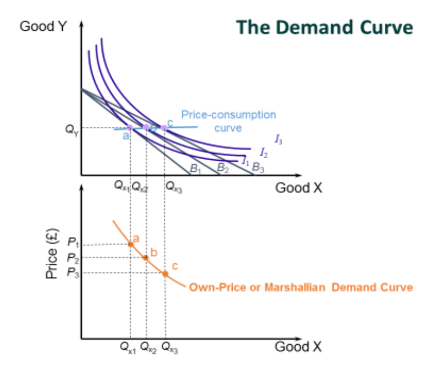
price offer and demand curves, for normal good

Suppose that we let the price of good 1 change while we hold p2 and income fixed. Geometrically this involves pivoting the budget line. We can think of connecting together the optimal points to construct the price offer curve. This curve represents the bundles that would be demanded at different prices for good 1.

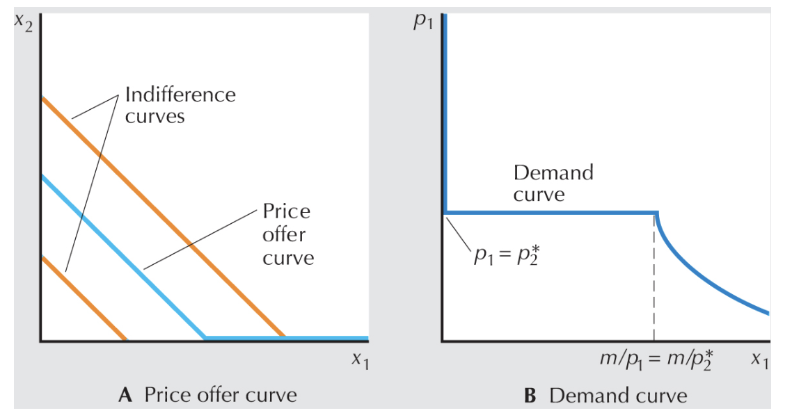
perfect subs, price offer curve and demand curve

The offer curve and demand curve for perfect substitutes—such as rival brands of sparkling water—. the demand for good 1 is zero when p1>p2, any amount on the budget line when p1=p2, and m/p1 when p1<p2. The offer curve traces out these possibilities.

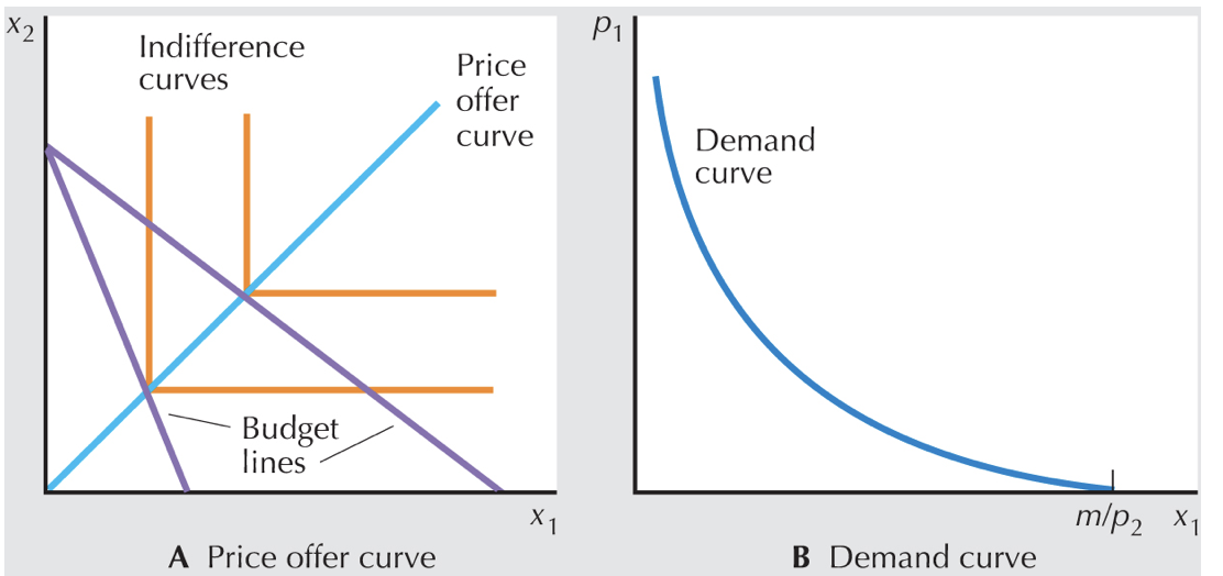
perfect complements, price offer curve and demand curve

The case of perfect complements—the right- and left-shoes example—. We know that whatever the prices are, a consumer will demand the same amount of goods 1 and 2. Thus their offer curve will be a diagonal line

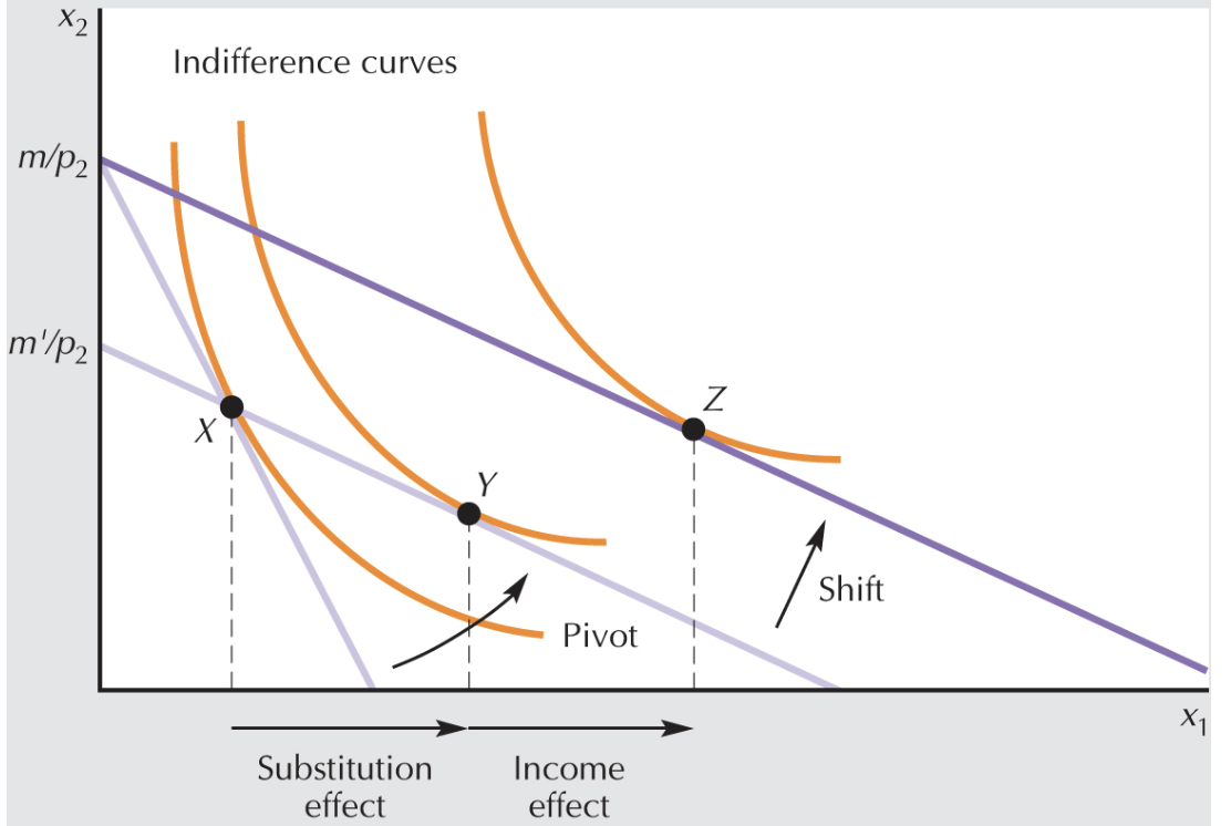
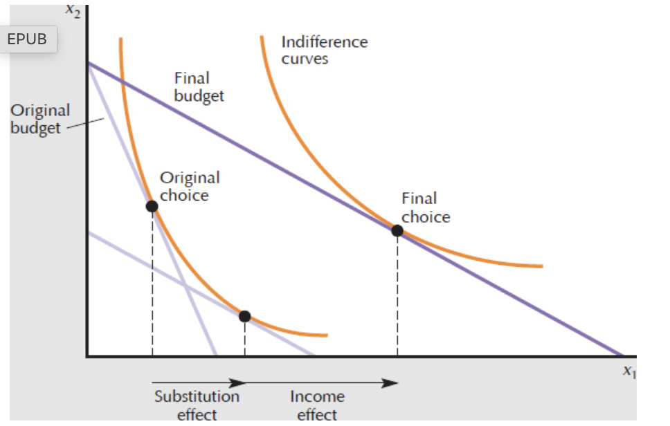
Slutsky decomposition income and sub effects, price fall

income is fixed, price of good 1 falls.

pivoted budget line by Y. This bundle of goods is the optimal bundle of goods when we change the price and then adjust dollar income so as to keep the old bundle of goods just affordable. The movement from X to Y is known as the substitution effect. It indicates how the consumer “substitutes” one good for the other when a price changes but purchasing power remains constant.

We turn now to the second stage of the price adjustment—the shift movement. We know that a parallel shift of the budget line is the movement that occurs when income changes while relative prices remain constant. this change moves us from the point (y1,y2) to (z1,z2). It is natural to call this last movement the income effect since all we are doing is changing income while keeping the prices fixed at the new prices.

When the price of a good decreases, we need to decrease income in order to keep purchasing power constant. If the good is a normal good, then this decrease in income will lead to a decrease in demand. If the good is an inferior good, then the decrease in income will lead to an increase in demand.

if a good is a normal good, then the income and substitution effects reinforce each other, so that the total change in demand is always in the “right” direction.

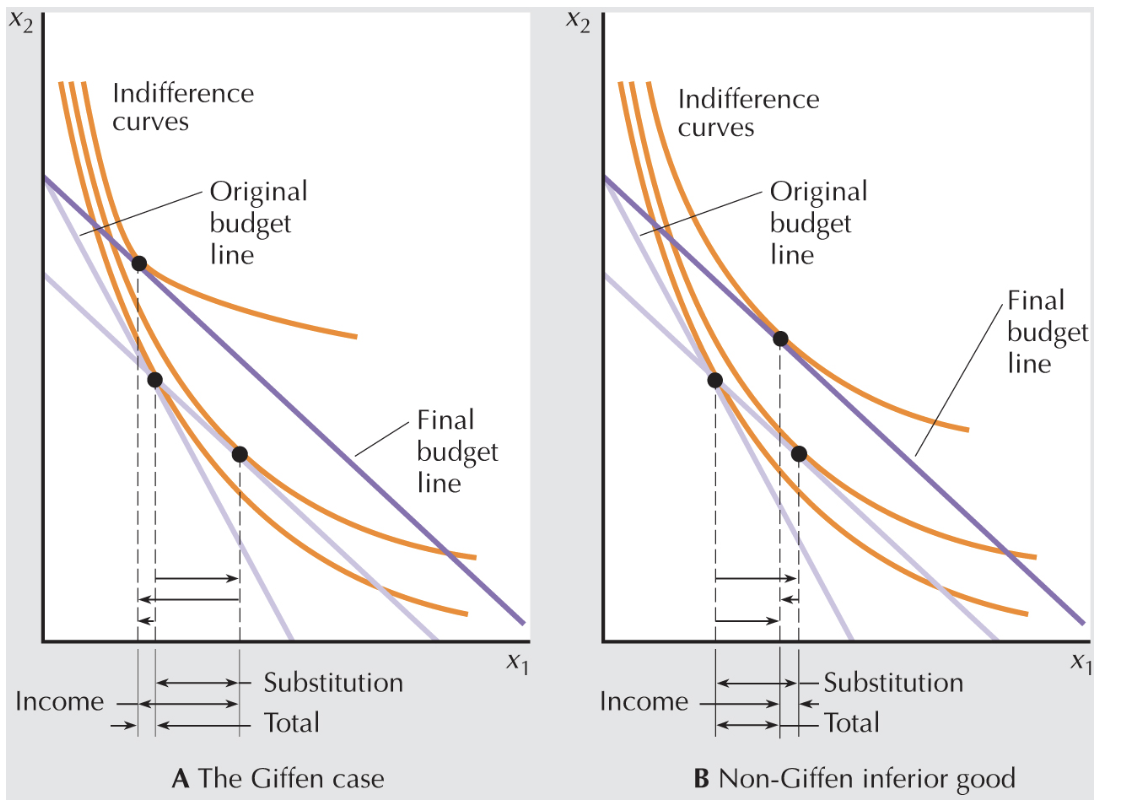
sub and income effect for inferior good, one giffen, one not.

for inferior goods, the income effect is negative, moves backwards

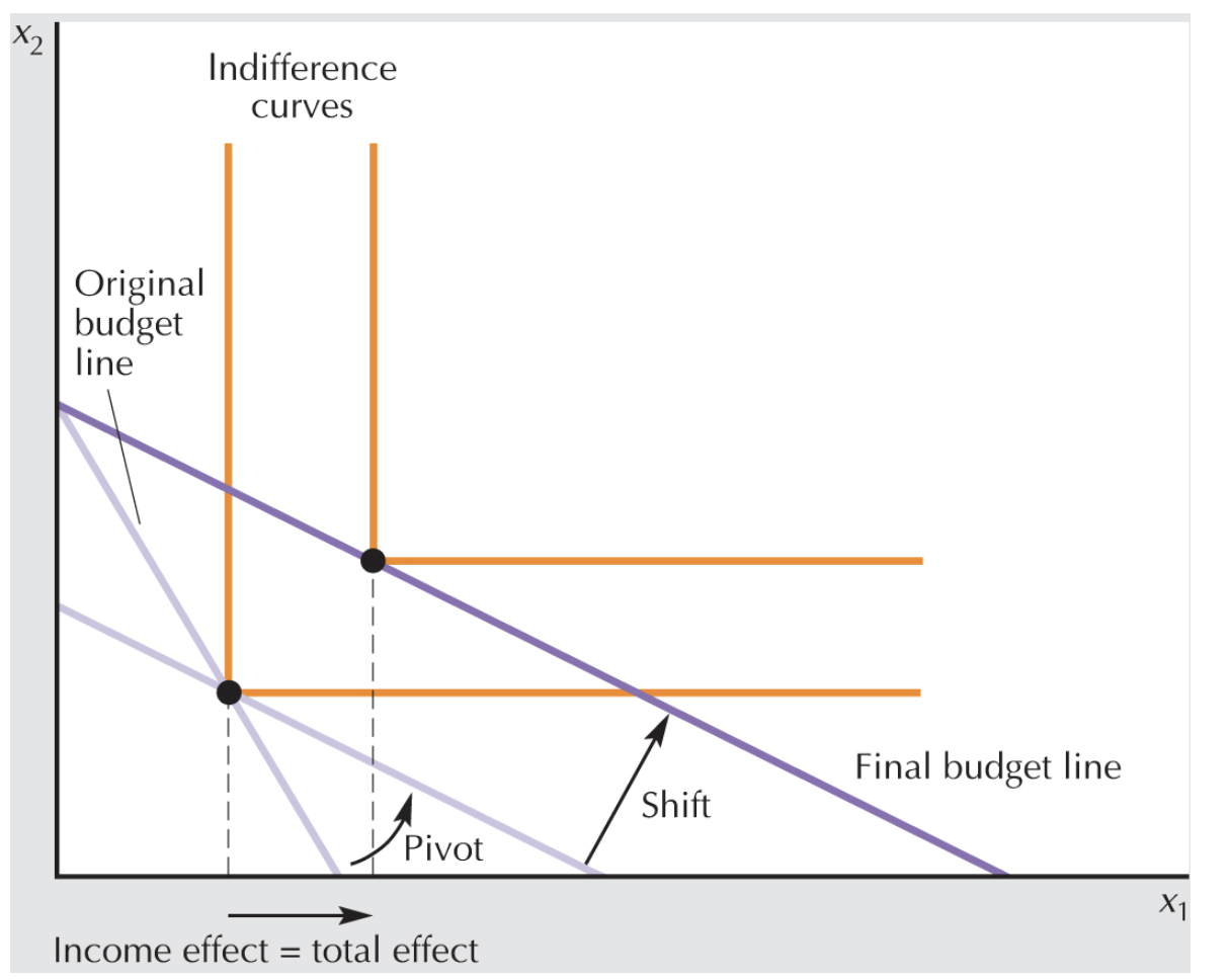
slutsky decomposition with perfect complements, good x1 price falls

When we pivot the budget line around the chosen point, the optimal choice at the new budget line is the same as at the old one—this means that the substitution effect is zero. The change in demand is due entirely to the income effect.

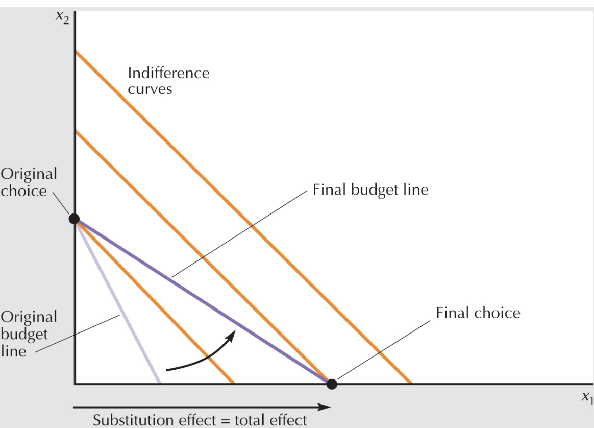
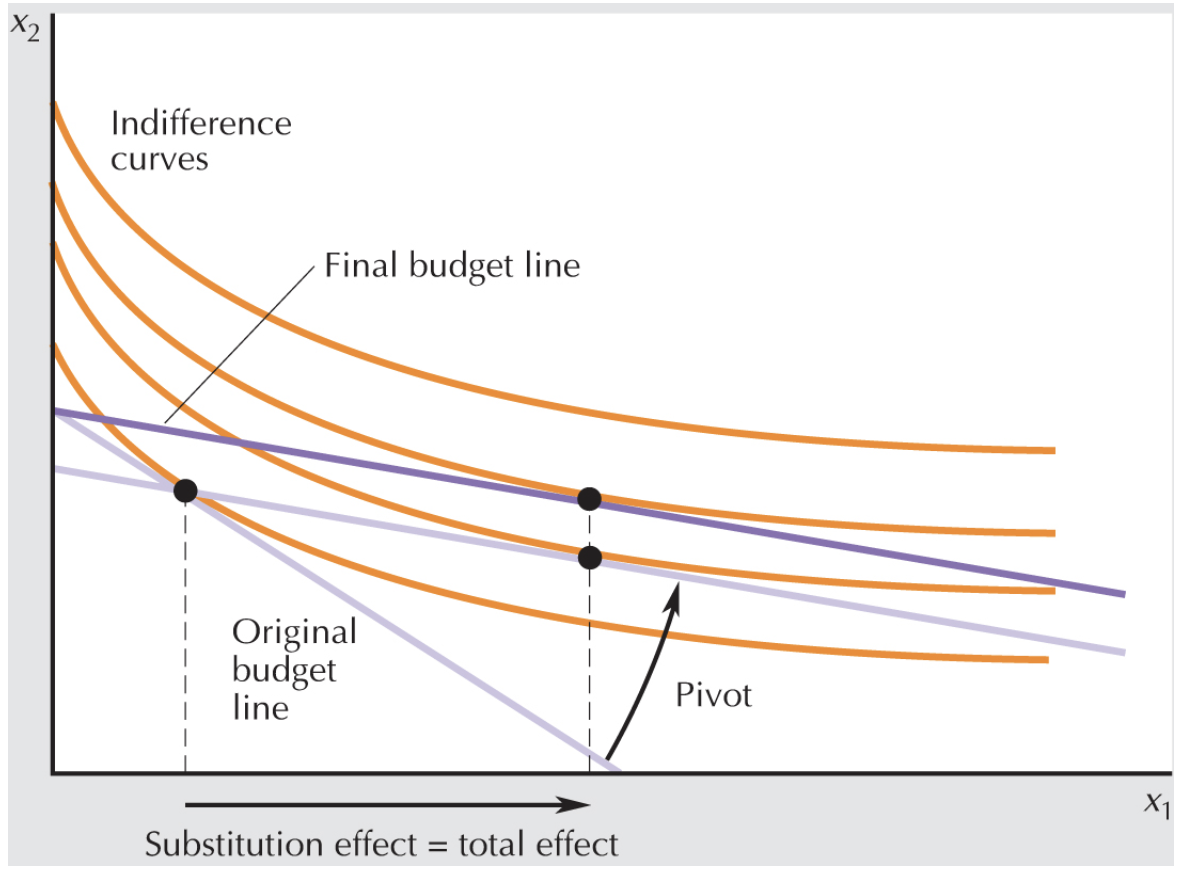
perfect subs, good x1 price falls

when we tilt the budget line, the demand bundle jumps from the vertical axis to the horizontal axis. There is no shifting left to do! In this case, the entire change in demand is due to the substitution effect.

quasi linear preferences slutsky decomposition, good x1 price falls

a shift in income causes no change in demand for good 1 when preferences are quasilinear. This means that the entire change in demand for good 1 is due to the substitution effect, and that the income effect is zero

A typical form is:

u(x1,x2)=v(x1)+x2

• You first choose the best amount of x1 based on prices

• Then you dump all remaining income into x2

So income only affects x2 not x1

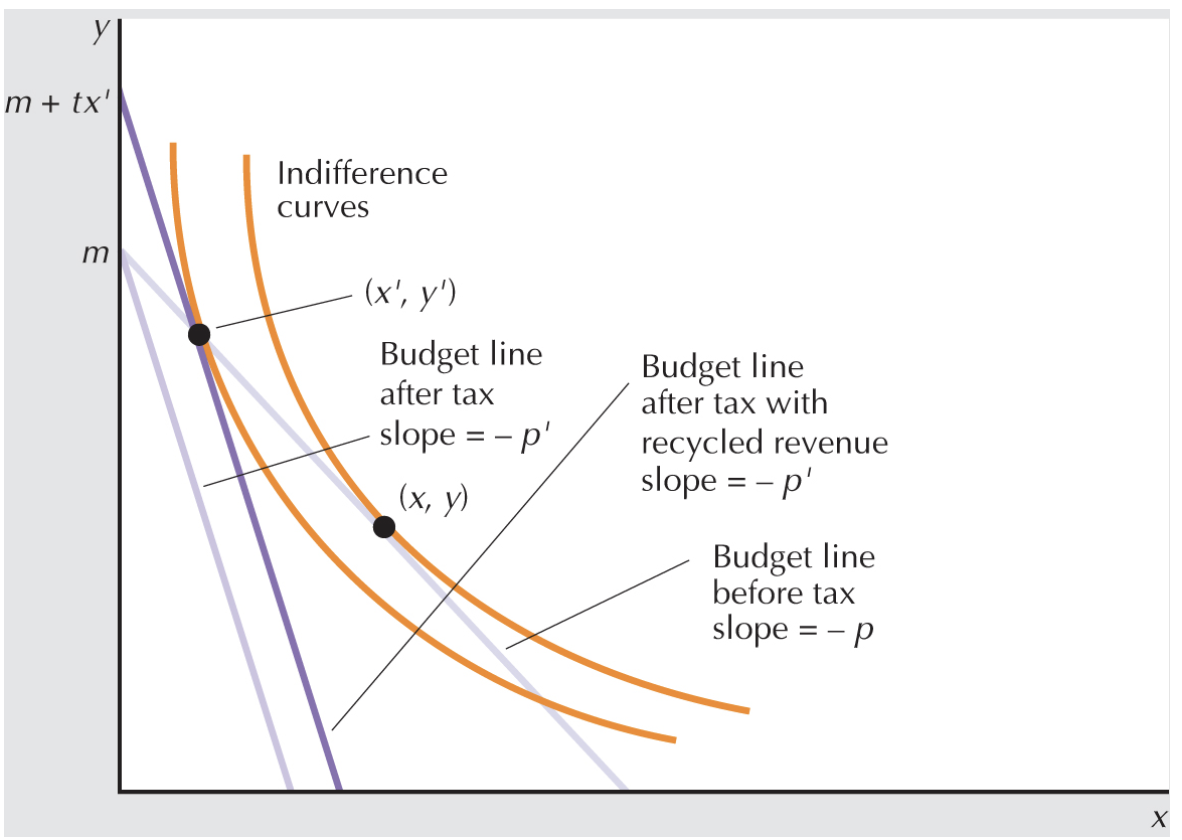
rwe, carbon tax and slutsky decomposition, when good x depends on the tax, good y doe not. so its same as an increase in price of good x

a tax t raises the price of the x-good from p to p′=p+t.The price change from (p,1) to (p′,1) will induce the average consumer to adjust their consumption from (x,y) to (x′,y′). The amount of revenue raised by this tax will be tx′.

The consumer’s original budget constraint,

p⁢x+y=m,

Without revenue recycling, the consumer’s budget line after the tax will rotate about the y-intercept. Recycling the revenue to the consumer produces an increase in income that shifts the budget line outward, without changing its slope.

The budget constraint with the recycled revenue is

(p+t)x’+y’=m+tx’ where tax rveenue is tx’

This example shows how revenue recycling, on its own, will not be enough to reverse the adverse consequences of the carbon tax.

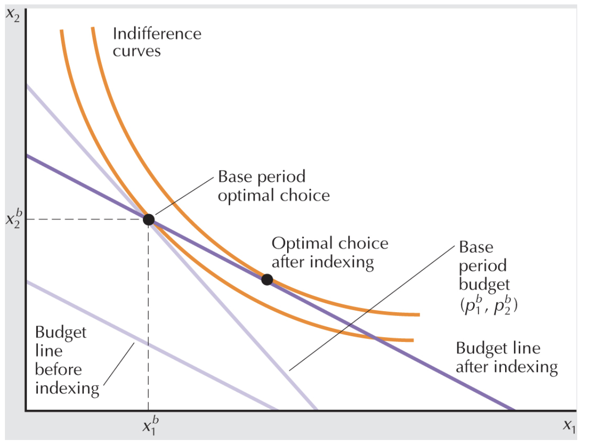
rwe changes in prices and indesximg, slutsky decomp

someone receiving social secuirty payemyns. price increases, but since some rise faster than others, ie in this case p2 price rises faster than p1. so busget line shifts inwards and slopechanges.

social secuirty payment incressdes to make initial bundle just as affordable as before. but now optimal bundle shifts.

Even though that bundle is still affordable at the new, higher prices, the substitution effect will induce the recipient to consume more of good 1 and less of good 2. And since the new budget line cuts through the old indifference curve, this consumption shift will be associated with a higher utility level. Thus, indexing Social Security payments by the CPI inflation rate more than compensates recipients for the adverse effects of price changes. This is called the substitution bias in the measurement of inflation: the CPI measure, using a fixed reference bundle, overstates the impact of price increases because it doesn’t take into account consumers’ shift away from goods whose prices rise faster.

hicksian effect, fall in prices

so to isolate sub effect, we wouild rotate, so m is still the same, but combos of x and y change cuz relative prices r different. then incomes also higher relative cuz of lower prices, so final choice is on a higher indifferent curve. but verbally, we can see how much income we can take away for them to have the same utility as before.

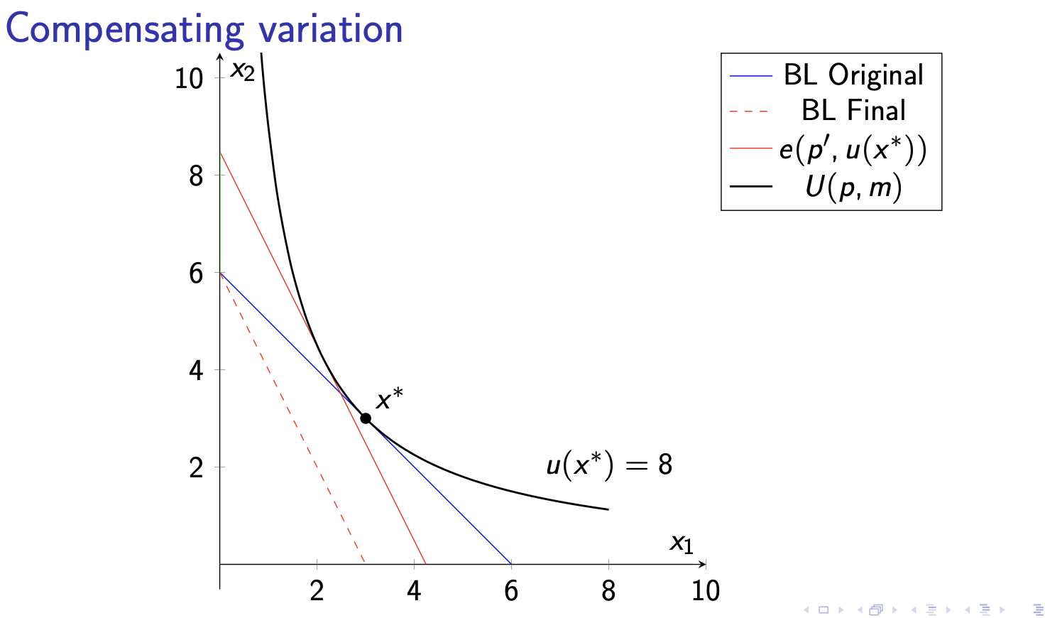
compensating variation

how do we get utility back to original, how much do we need to compensate due to price rise. how much to pay to be just as happy as befpore.

BL original is the original line before price rise.

BL final shows lower IC due to price rise.

To compensate we shift to obtain same IC at new slopes. the red line.

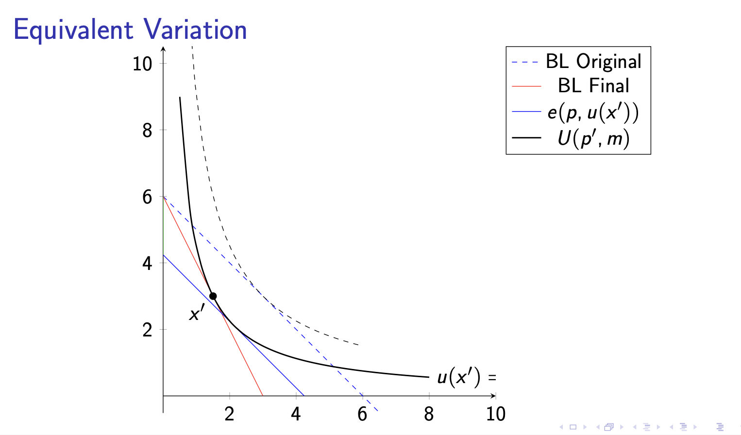
equivalent variation

parallel shift from the original budget constraint. we are looking at bhow much we have to take away to be as worse off as u are after the price change, using old prices. so cuz we’re using old prices we need original slope therefore original budgent cosntaraint.

theoretically EV=CV, what youd lose if something bad happens (EV) is equal to what youd accept to ensure it (CV)

in reality, CV tends to be higher cuz of loss aversion bias, because we tend to assess losses as being worse than equivalent compensation.

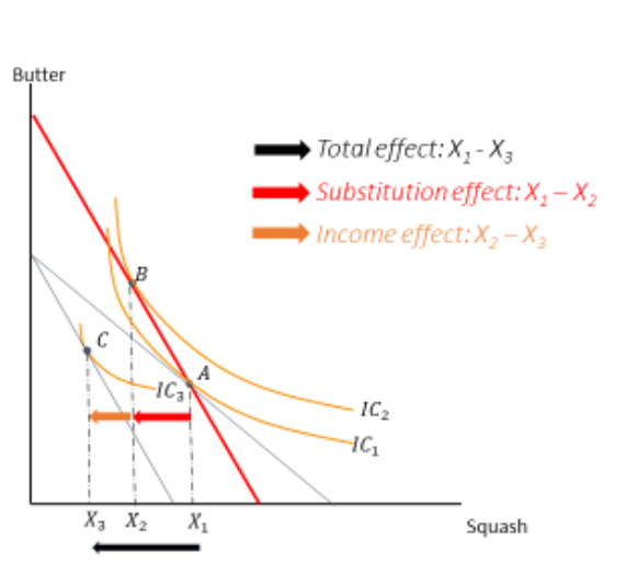
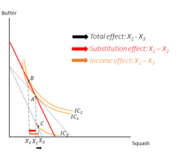
slutsky decomp with good price rise for normal good

• Start at utility maximisation on IC1 at point A

• Price of squash rises → budget constraint pivots inward

• New optimal bundle (with income + substitution effects) is at point C

• To separate effects using Slutsky, keep purchasing power constant

• Draw compensated budget line:

  • Same slope as new budget line (reflects new price ratio)

  • Passes through original bundle A

• Utility maximisation on this compensated line gives point B

• Movement from A → B = Slutsky substitution effect

  • Squash becomes relatively more expensive

  • Consumer substitutes away from squash → consumption falls

• Movement from B → C = income effect

  • Price rise reduces real income

  • Since squash is a normal good → demand falls further

• Total effect (A → C) = substitution effect + income effect

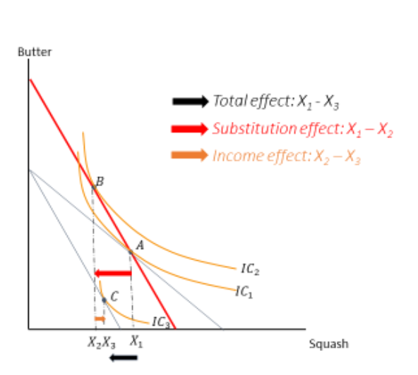
slutsky price rise inferior, non giffen

• Substitution effect is unchanged from normal good

• Price of squash rises → substitution effect still reduces consumption (A → B)

• Squash is now an inferior (non-Giffen) good

• Price rise → real income falls

• For an inferior good → lower real income increases demand

• Income effect (B → C) increases consumption of squash

• Income effect works in the opposite direction to substitution effect

• However, squash is not a Giffen good

• Substitution effect is larger than income effect

• Overall effect (A → C) is a fall in quantity demanded

• Final quantity at C is lower than original quantity at A

slutsky price rise inferior, giffen

• same sub effect as others

• Price of squash rises → substitution effect reduces consumption (A → B)

• Squash is now a Giffen good (strongly inferior)

• Price rise → real income falls

• For a Giffen good → lower real income increases demand significantly

• Income effect (B → C) increases consumption of squash

• Income effect works in the opposite direction to substitution effect

• Income effect is larger than substitution effect

• Overall effect (A → C) is an increase in quantity demanded

• Final quantity at C is higher than original quantity at A

Marshallian demand curve when utility function follows normal form: U(x)=X^aY^1-a when price of good x falls. assume X is a normal good

The own-price or Marshallian demand curve is derived below for a normal good. The Marshallian demand curve takes account of both substitution and income effects. With a normal good, both effects work in the same direction, so following the fall in price, demand for good X will rise.

Hicksian demand curves (sub effect) for normal inferior or giffen good following price rises and falls

Hicksian demand curve implies we are only looking at the change due to the substitution effect (keeping utility constant). Irrespective of the good, the substitution effect always works in the same direction – a fall in the price of Good X will cause the quantity to rise (vice versa for price rise). The diagram below shows you how to derive Hicksian demand if there is a price fall and a price rise. Both give exactly the same curve, but as you can see in the top diagram, the budget constraint pivots in the opposite direction.

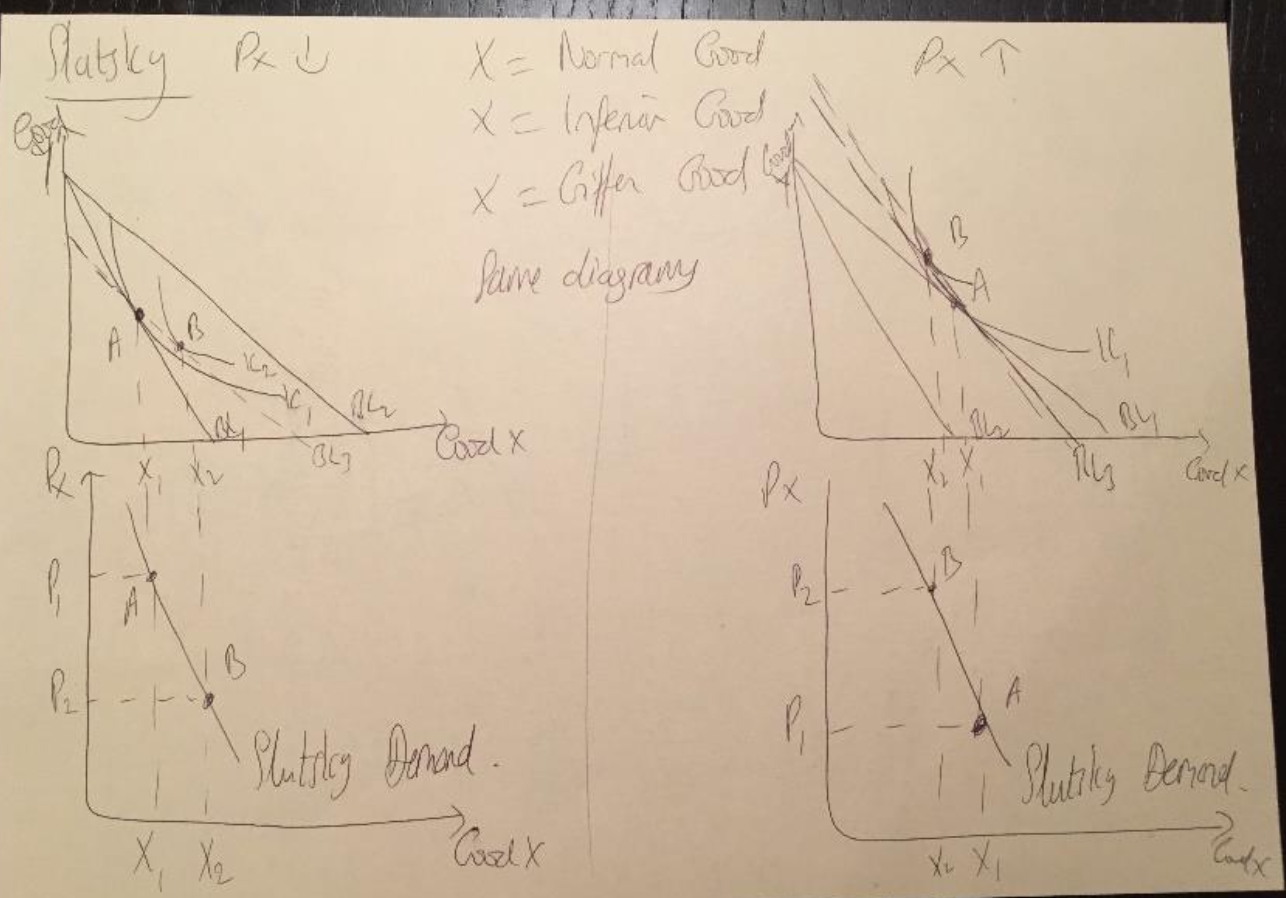
Slutsky demand curves (sub effect) for normal inferior or giffen good following price rises and falls

we are again only looking at the change due to the substitution effect, but this time we are keeping purchasing power constant. Again, irrespective of the good, the substitution effect always works in the same direction – a fall in the price of Good X will cause the quantity to rise (vice versa for price rise)

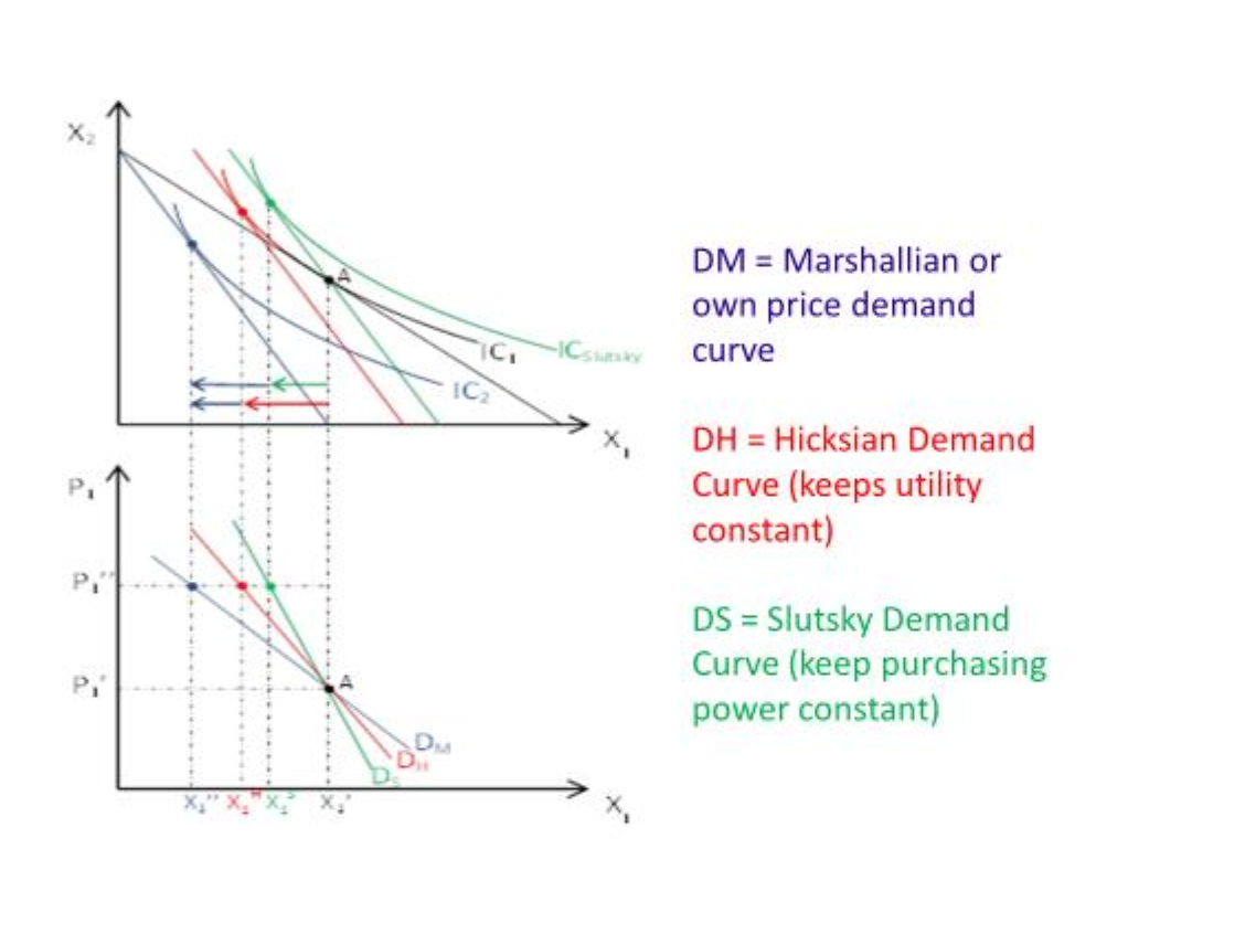
Marshallian, Hiskcian, and Slutsky demand curves for rise in price of good X. normal good

Slutsky demand is steepest because it fully compensates purchasing power (removing most of the income effect), Hicksian is intermediate as it maintains utility, and Marshallian is flattest because it includes both income and substitution effects.

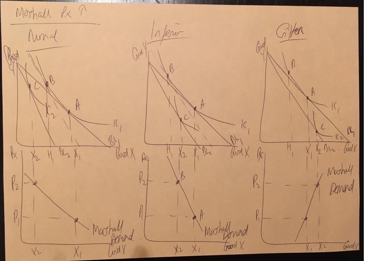
Marshallian demand curve for inferior giffen, inferior non giffen, and normal

For a Giffen good, the Marshallian demand curve slopes upwards, as now the

income effect more than offsets the substitution effect, hence following the fall in

price the quantity of X actually falls.

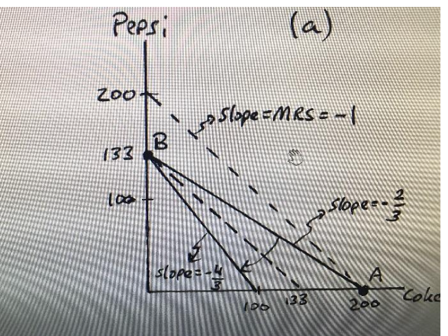
perfect subsittues, rise in price of good x1.

• Goods are perfect substitutes → indifference curves are straight lines

• Marginal rate of substitution (MRS) is constant at -1 (1:1 trade-off)

• Budget lines are straight with slope = relative price ratio

• Original budget constraint slope = -2/3 (Coke relatively cheaper)

• Optimal bundle at A → consume only Coke (corner solution) cuz this is highest attainable IC

• Price of good 1 (Coke) rises → new budget slope = -4/3 (Coke now relatively more expensive)

• Budget line becomes steeper than indifference curves

• New optimal bundle at B → consume only Pepsi (corner solution), highest attainable IC

• Intuition:

  • When Coke is cheaper → buy only Coke

  • When Coke becomes more expensive → switch entirely to Pepsi

if same price, solid and dashed line intersect so all optimal bundles.

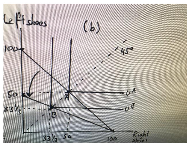
perfect complements, price increase of good 1.

• Goods are perfect complements → L-shaped indifference curves

• Must be consumed in fixed proportions (1:1 pairs)

• Optimal choice always occurs at the kink

• Price of left shoes rises to £2

• Budget constraint pivots inward

• New vertical intercept = 50 (left shoes more expensive)

• New optimal bundle at B (still at kink)

• Consume 33.3 left shoes and 33.3 right shoes

• Key intuition:

  • Goods must be used together → no substitution possible

  • Increase in price of one good reduces consumption of both goods equally

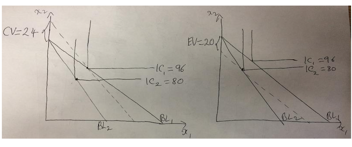
equivalent and compensating variation following a price rise of good x. they are perfect complements,

CV: how to maintain old utility, . oEV: old prices so same budget constaint slope, new utility.

the compensating variation is higher than the equivalent variation, showing the amount of compensation that has to be paid at the new higher price is more than at the original lower price. They are different as £1 is worth differing amounts at different prices and is worth less at higher prices.

coase theorem MWTP

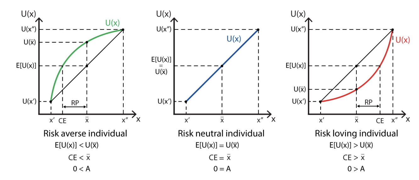
risk aversion, neutral, and seeking

RP is risk premium

MWTP public good (ie I listen to music, it affects neighbour)

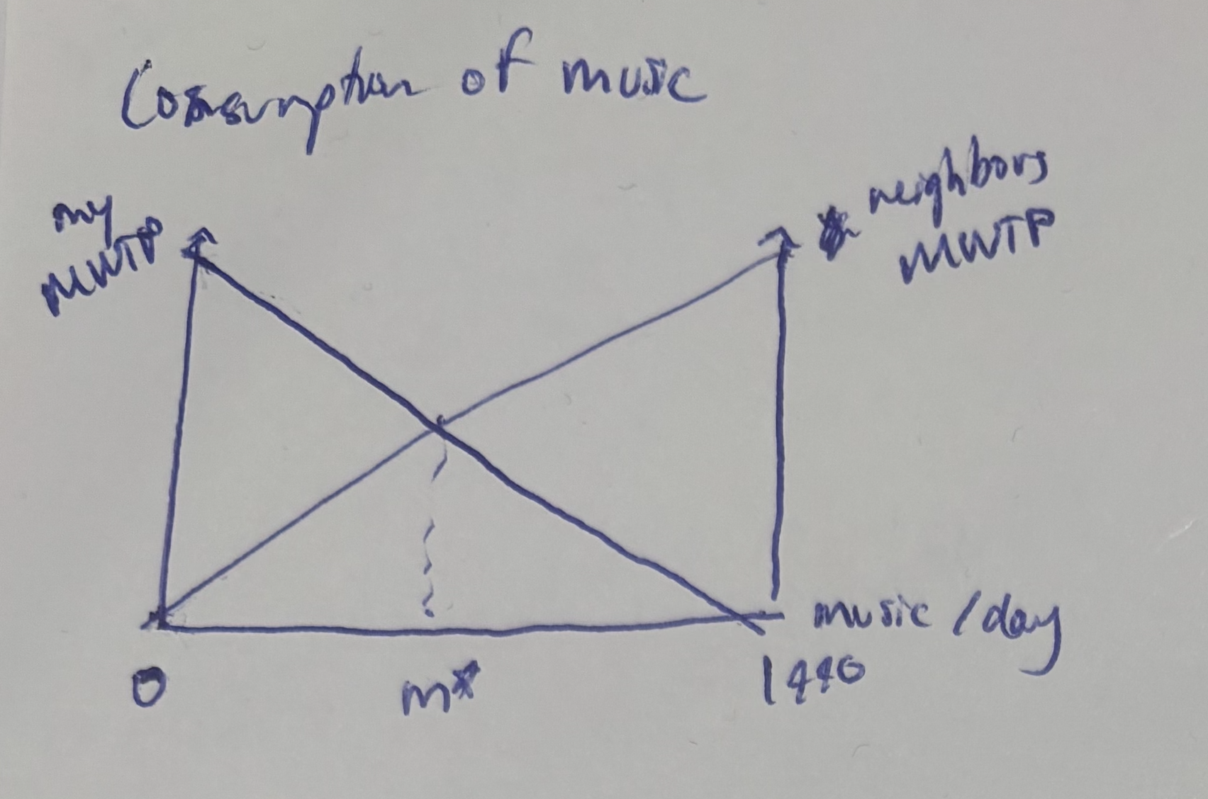
different levels of public good and their MC/MB. Ie cinema vs fireworks

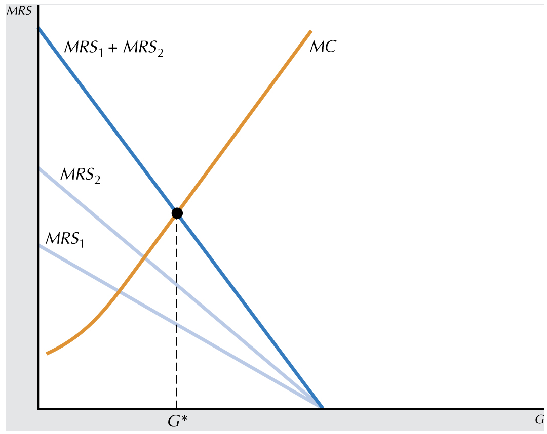
Public good efficient allocation

where vertical sum of the MRS, or MWTP, equals the MC

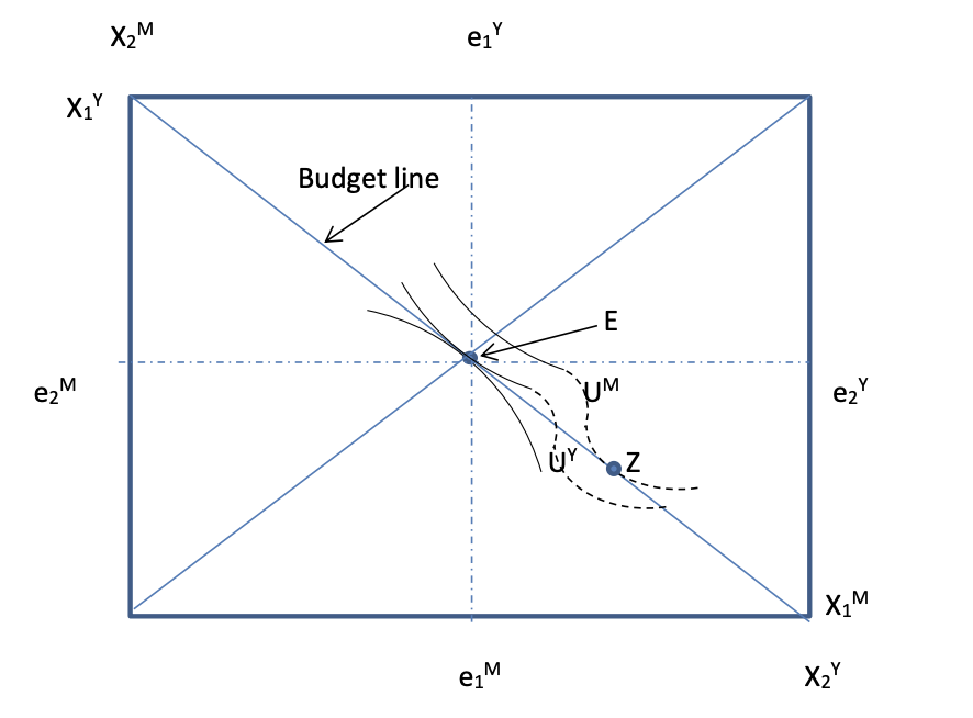
edgeowrth box with equal initial endowments, equal MRS of -1

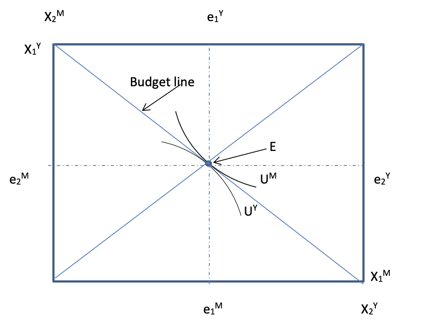
edgeworth box introducing non ceonvexity, there is efficiency, but no longer a competitive equilbirium

E is still efficient, but when faced with the budget line that previously supported E as an equilibrium, I now no longer optimize at E, as I can now get to a higher indifference curve and would want to optimise at point Z. Therefore if tastes are allowed to be non-convex the existence of a competitive equilibrium in an exchange economy cannot be guaranteed. The degree of convexity does mean that E could still be the competitive equilibrium, but it can’t be guaranteed.

Consider two goods X (Pasta on the horizontal axis) and Y, Coffee. Start with a given budget constraint and then explain/show what will happen to the budget constraint if: (a) The government imposes a quantity tax (t) on coffee? (b) The government imposes a lump sum tax? (c) The government rations pasta to 𝑥̅? (d) The government imposes a tax, t, on pasta consumed beyond 𝑥̅? (e) The consumer receives an in-kind transfer of 40g of pasta?

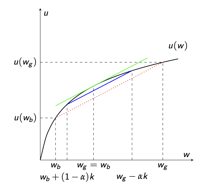
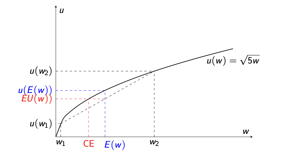
U(EW) vs E(U(EW))

full insurance, wb, wg graphically