Stats One-way Between-subjects ANOVA

ANOVA recipe book

1. Choose one IV and the DV

2. Calculate how many independent t-tests you need to run (Number of t-tests = k(k-1) / 2

3. Problem with testing the same ingredient multiple times: Capitalising on chance (increase risk of Type I error as a result of running many statistical tests on the same data)

4. Give one specific type of Type I error that could occur if multiple independent t-tests were run

5. Calculate the cumulative probability: P (at least one Type I error) = 1 - (1 - a)ⁿ Where n = number of independent-samples t-tests

6. Based on the cumulative probability of making at least one Type I error, explain what this value means (e.g. there is a 14.3% chance this is significant by chance

7. Between-groups variance = between between groups (treatment + error) / Within-groups variance = variance WITHIN the same group (error)

Assumptions of one-way between-subjects ANOVA

1. Levels of measurement = continuous DV

2. Independence = Each observation is independent of the others (each score should come from a different participant)

3. Normality of residuals = Normally distributed residuals along the reference line of a QQ plot

4. Homogeneity of variance = All groups being compared have equal variability / The spread of scores around the mean is approximately the same across both groups

• Boxplot

• Residuals vs Fitted plot (flat red line)

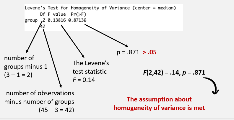
• Levene’s Test → F = .xx, p = .xxx

What happens if the assumptions are violated? (Non-parametric test)

Kruskal-Wallis test for non-parametric test

If groups have equal sample sizes and the effect sizes are relatively large, you can proceed with ANOVA despite violations of assumptions

“Heterogeneity of variances is always a problem in ANOVA, even in the moderate heterogeneity cases. Welch's method is most popular procedure to analyse the data with different variance values. However, this method performs better solution in the assumption of normality like other traditional methods"

Eta squared

ANOVA’s effect size - Ranges from 0 to 1

For one-way between-subjects designs, partial eta squared is equaivalent to eta squared

Eta squared links to total variance, partial eta squared links to variance related to the treatment

• Eta squared = 0.01 indicates a small effect

• Eta squared = 0.06 indicates a medium effect

• Eta squared = 0.14 indicates a large effect

Write up

A one-way between-subjects ANOVA was conducted to examine whether learning motivation differed across study-with-me conditions

The analysis revealed a significant effect of condition on learning motivation, F(2, 42) = 15.17, p < .001, [partial eta squared] = 0.42, indicating that learning motivation differed significantly across the three conditions

• F(x, xx) = x.xx, p < .xx, [partial eta squared] = x.xx

Omnibus test definition

Omnibus test (e.g. ANOVA) - Tests for the significance and acts as a global check (e.g., ANOVA, regression -test) - detects if one group mean differences from the other (variance) without saying which groups are specifically different

Post-hoc test definition

• Post-hoc tests are conducted only after a ANOVA test shows a statistically significant result 

• Post-hoc tests are used to identify group differences by comparing every group in the study against all other groups

• Popular post-hoc tests are Tukey, Bonferroni and Scheffé 

• Keeps the alpha level consistent at 0.5 AND can be used for multiple comparisons (avoiding capitalising on chance)

Post-hoc test for one-way between-subjects ANOVA

Tukey’s Honestly Significant Difference (HSD)

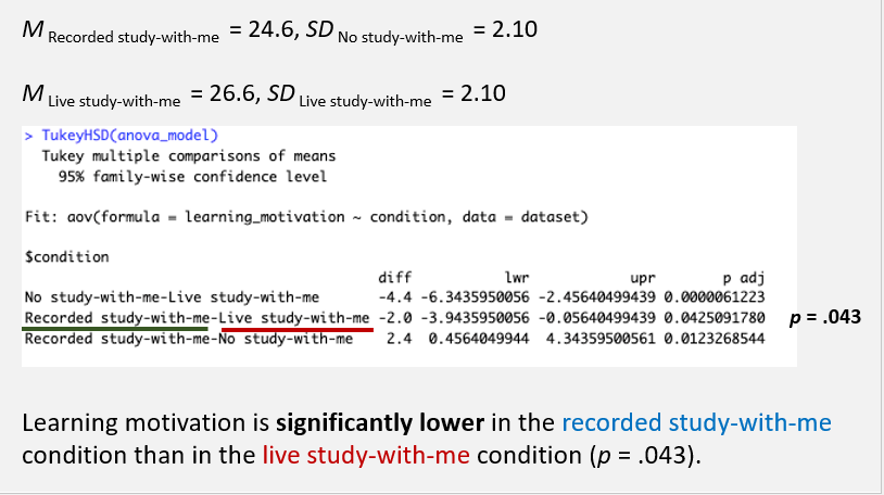
TukeyHSD(anova_model)

Look at p adj and see if the significance is lower than .05 (or your chosen significance score). Which mean score of the IV was lower than the other?

In this example, because Mean Recorded study-with-me was lower than the Mean Live study-with-me AND the p-value was lower than .05, learning motivation in recorded study-with-me is therefore SIGNIFICANTLY LOWER than live study-with-me

Write up: Post-hoc comparisons using Tukey’s HSD test revealed that learning motivation was significantly higher in the live study-with-me condition than in both the recorded study-with-me (p = .043) and no study-with-me conditions (p < .001). In addition, learning motivation was significantly higher in the recorded study-with-me condition than in the no study-with-me condition (p = .012)

• p = .xxx

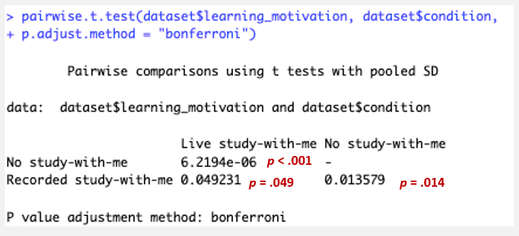
Bonferroni: Another post-hoc test

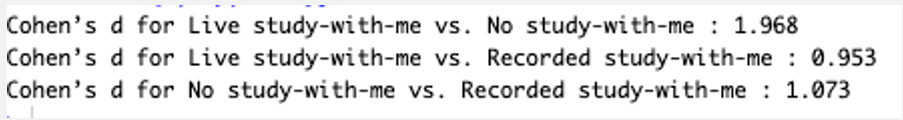
There are two effect sizes for ANOVA: Eta-equared and Cohen’s d for pairwise comparison

pairwise.t.test(x$x, x$x, p.adjust.method = "bonferrroni")

Write up: Post-hoc comparisons using Tukey’s HSD test revealed that learning motivation was significantly higher in the live study-with-me condition than in both the recorded study-with-me (p = .043, Cohen’s d = 0.95) and no study-with-me conditions (p < .001, Cohen’s d = 1.97). In addition, learning motivation was significantly higher in the recorded study-with-me condition than in the no study-with-me condition (p = .012, Cohen’s d = 1.07)

• p = .xxx, Cohen’s d = x.xx