S2 L2 Multi choice models

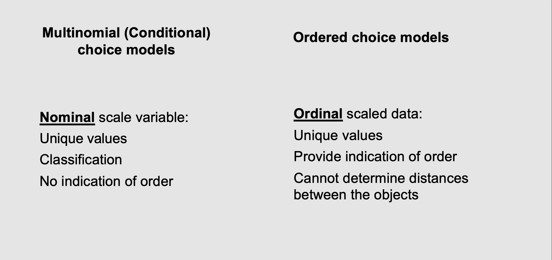
What are the types of mutilpe choice data (2)

• What it means: When you have more than two choices, the data can take two different forms. You have to know which one you are dealing with because the computer uses different math for each :

  1. Nominal scale (Multinomial Models): The choices are just different categories with no mathematical rank or order . For example, a Bus isn't mathematically "higher" or "lower" than a Train; they are just different classifications.

  2. Ordinal scale: The choices do have a natural order . Think of a customer satisfaction survey: "1 - Unhappy, 2 - Neutral, 3 - Happy." You know that 3 is better than 1, but you don't know the exact, precise mathematical distance between "Neutral" and "Happy" .

• The takeaway for this lecture: This specific lecture is entirely focused on Nominal data. We are learning how to model human choices between completely unranked categories (like choosing a brand of cereal, or deciding which transport mode to take).

What is a Mutlinomial logit model (MNL)

• What it means: The professor brings back the Random Utility equation: Total Happiness ($U$) = Measured Facts ($V$) + Unmeasured Randomness ($\epsilon$). But to make the computer solve it for multiple choices, we have to assume the randomness ($\epsilon$) follows an "extreme value" distribution .

• Real-world translation: If you only have two choices, assuming human randomness follows a standard "bell curve" is easy. But if you have 4 or 5 choices, calculating overlapping bell curves crashes the math. The "extreme value" distribution is just a mathematical shortcut that gives the computer an equation it can actually solve.

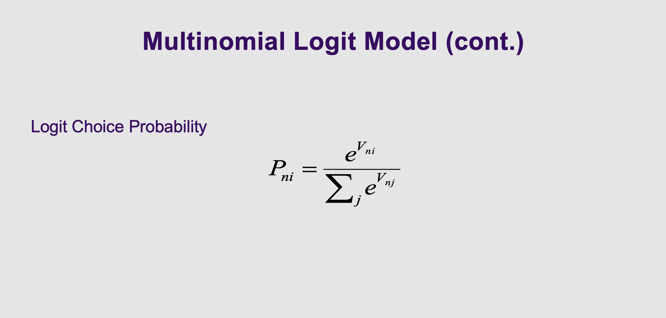
What is the clean probability fomrula for MLM

• What it means: This is the final, clean probability formula . The probability of picking option $i$ equals $e$ raised to the utility of $i$, divided by the sum of $e$ raised to the utility of all options.

• Real-world translation: Why do we use '$e$'? Let's say a train ticket costs £500. Its happiness score ($V$) might be highly negative (e.g., -5). But a probability can never be negative (you can't have a -20% chance of taking the train). In math, raising '$e$' to any power—even a negative one—always creates a positive number. This brilliant trick ensures all your probabilities stay positive!

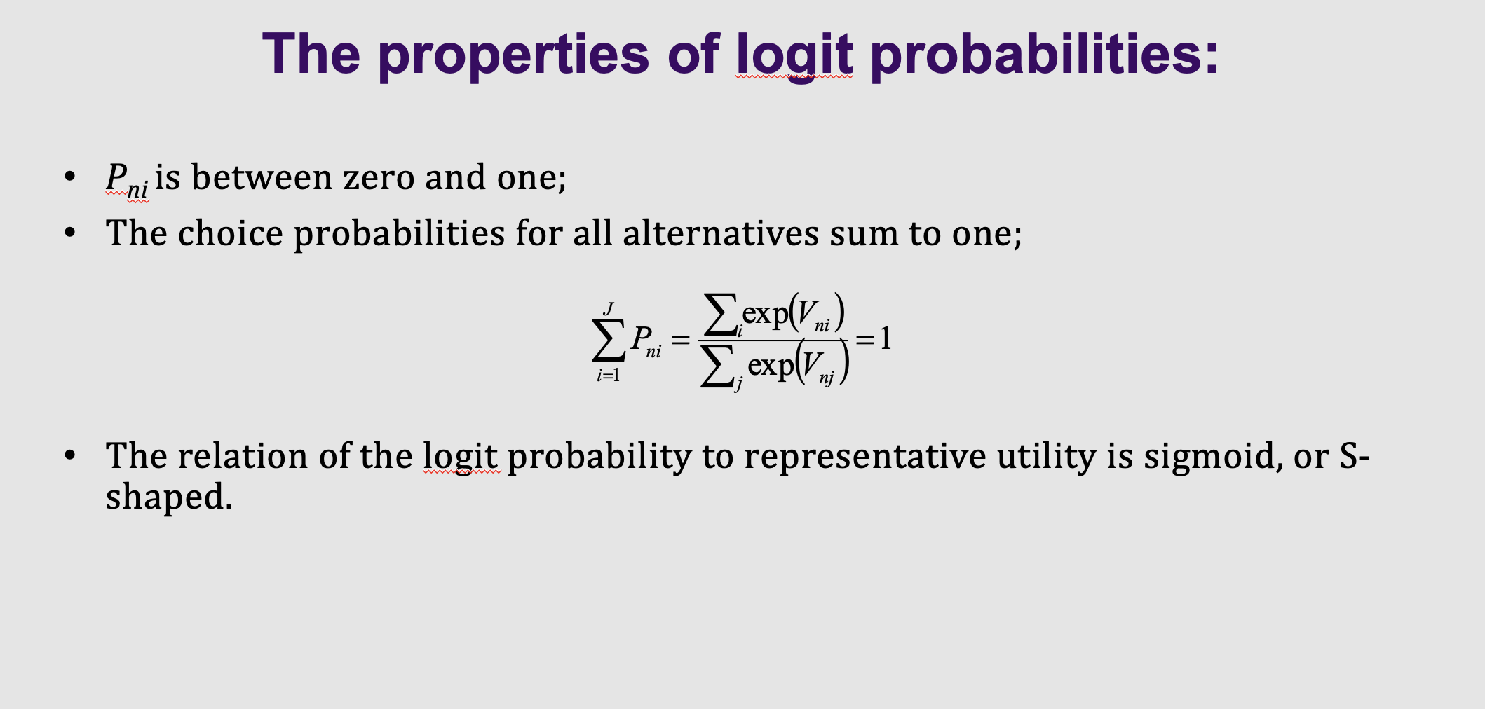
What are the properties of the logit probabilities

What it means: Because of the formula on Slide 6, the model follows three strict rules :

1. Every probability is between 0 and 1.

2. If you add up the probabilities of every option, they perfectly sum to 1 (100%).

3. The curve is S-shaped (Slide 8 shows this visually) .

What are the four estimations we have to make?

What it means: Because we are using S-curves instead of straight lines, we have to use Maximum Likelihood Estimation (MLE) to find the answers . The computer uses trial and error to find the coefficients that make your observed data most likely to happen.

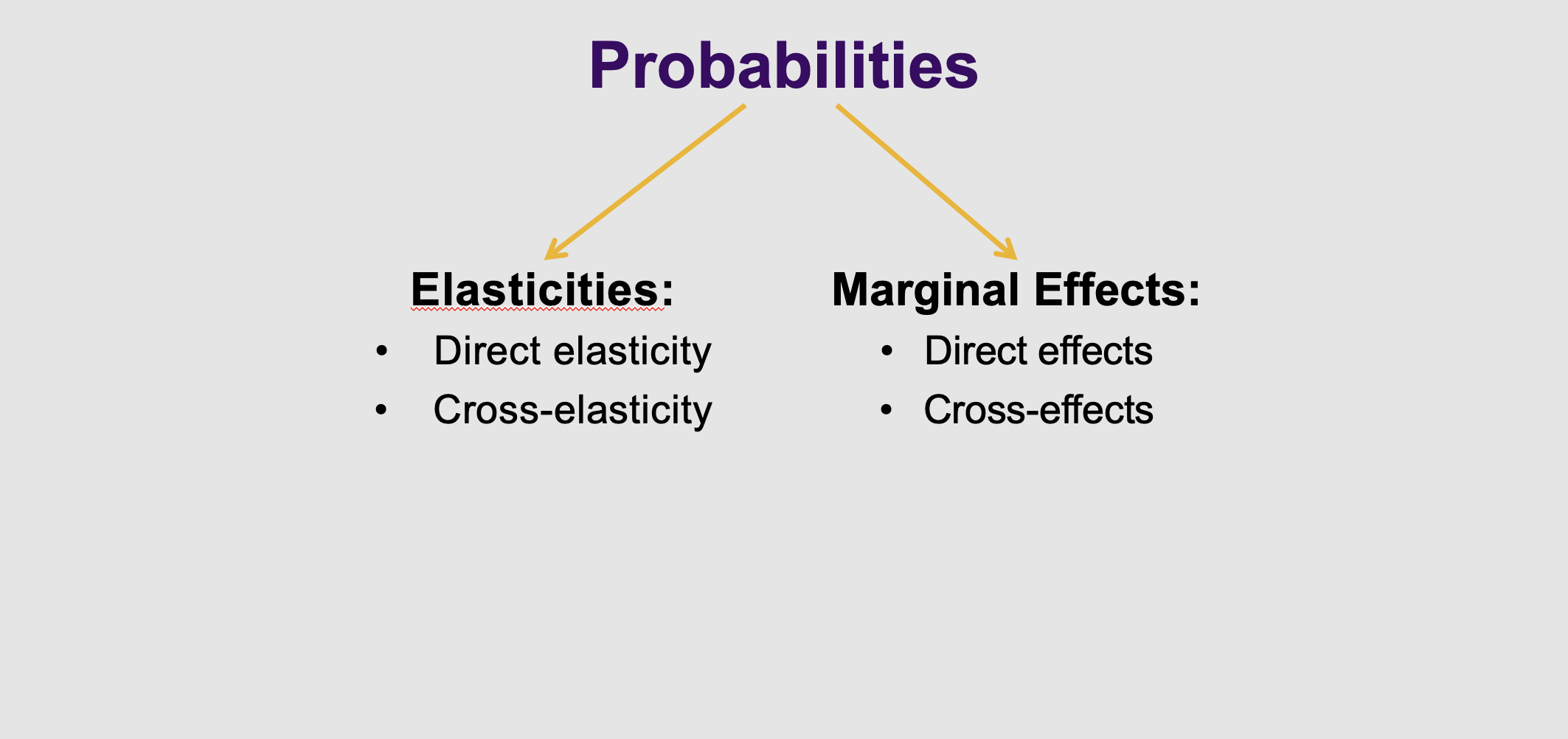
What are the two outcomes of probabilities we can use

• What it means: When the computer finishes its MLE trial and error, it spits out raw numbers (coefficients). Because S-curve math is so weird, those numbers are meaningless to humans. We have to translate them into Marginal Effects, which measure absolute changes .

• Real-world translation: * Direct Effect: If the price of the bus goes up by £1, the absolute probability of taking the bus drops by 2%.

  • Cross Effect: If the price of the bus goes up by £1, the absolute probability of taking the train increases by 1%.

What do both of these mean

Direct - increase the quality of the bus service to work, what is the impact of this

 

Cross - taking the alternatives changes a unit change

Prob of taking the bus changes when the quality of the train changes

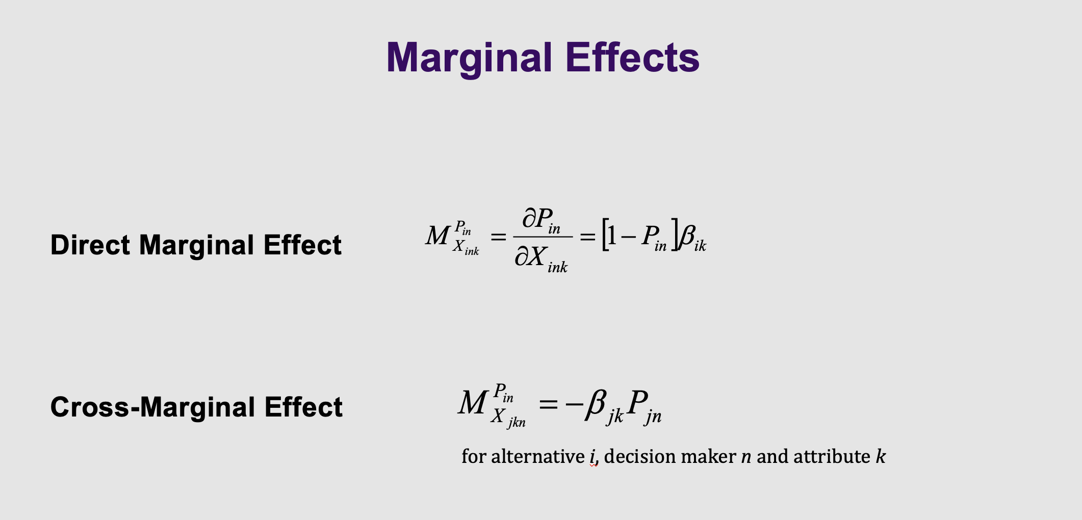
What are the formulas of the direct and cross effects

• What it means: Economists prefer percentages over absolute numbers, so they use Elasticities instead .

• Real-world translation: * Direct Elasticity: If the bus gets 10% more expensive, the probability of taking the bus drops by X%.

  • Cross Elasticity: If the bus gets 10% more expensive, the probability of taking the train increases by Y%.

What can we use to see how well the model fits?

What it means: You cannot use standard $R^2$ to grade an S-curve model. You have to use a Pseudo R-squared or Likelihood Ratio Index . This grades your model by comparing it to a "dumb" baseline model (a model with no variables, just alternative-specific constants) to see how much your variables actually helped predict the choice .

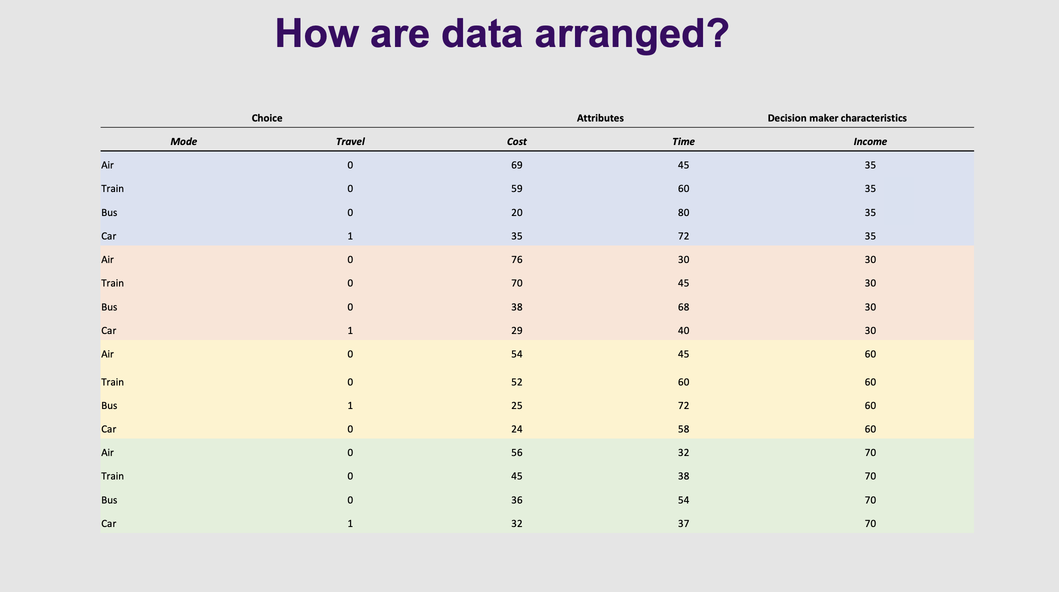
How is the data for the air,train, bus and acr arranged

Real-world translation: Look closely at the table on Slide 18. Notice how one person takes up 4 rows! Every single option gets its own row, and a 1 is placed next to the mode they actually chose .

Data is arrange slightly different. Here each individual will have as many row as there are alternatives . Each colour is a different individual. Dependent variable is travel, cant have more than one, 1, in the same block colour unless it is continued over time. Explanatory variables - cost and time. Income doesn’t vary across alternatives, can't calculate co efficient when there is variation across alternatives

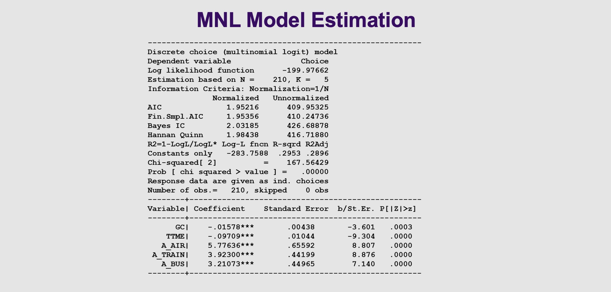
What do we look for in the MNL model outputs

Three alternatives, car is the base category.

 

Fit of the model

• Log likelihood function, when it reaches a maximum. If you add variables and increase, better fit

• Constants only, log ratio index

• Chi squared is the log ratio index

  • Has a p value attached,

 

GC and time are negatively related and significant.

What it means: This is what the software prints out . Notice the coefficients for Cost (GC) and Time (TTME) are negative. This makes logical sense—as travel time and cost go up, your desire to take that mode goes down!

How do you determine Direct and Cross elasticitie

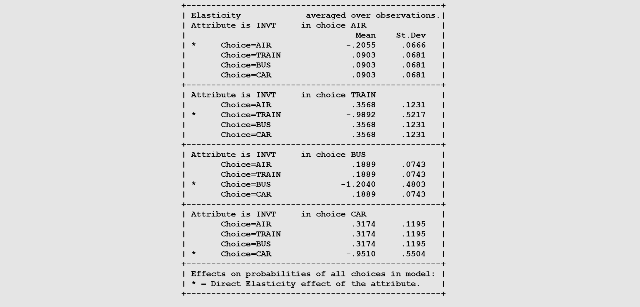
• What it means: Here is the readable translation (Elasticities). Look at the box for "Choice AIR" .

• Real-world translation: * The Direct Elasticity (with the asterisk) is -0.2055. If flying takes 1% longer, the probability of flying drops by 0.20%.

  • Look at the three Cross Elasticities below it. They are all exactly 0.0903! This is a massive mathematical flaw in the model that leads directly to the next slide.

What are the limitations of the logit model? (3)

: IIA means the model mathematically forces the ratio of probabilities between any two choices to stay exactly the same, no matter what other choices are added to or removed from the mix.

1. "Taste" Variation

• What it means: The standard MNL model assumes that everyone in your dataset has the exact same "taste" or preference weights for the attributes. For example, it assumes every single commuter hates a £1 price increase equally.

• The Reality: Human tastes vary wildly! A wealthy executive might not care about a £5 ticket increase, while a college student might switch to walking immediately. The basic MNL model struggles to capture these random, individual differences in taste unless you have highly detailed demographic data for every person.

2. Substitution Patterns

• What it means: This is actually the root cause of the Red-Bus-Blue-Bus problem we talked about. The MNL model uses extremely rigid, proportional substitution patterns. If one option becomes unavailable (or a new one is added), the model assumes people will substitute to all the other options in exact proportion to their existing market shares.

• The Reality: Substitutions in the real world are messy and clumped. If the train breaks down, train riders don't distribute evenly across planes, cars, and walking; they almost all substitute to the bus because it's the closest alternative. The standard MNL model cannot handle these flexible substitution patterns.

What is the red bus blue bus example problem

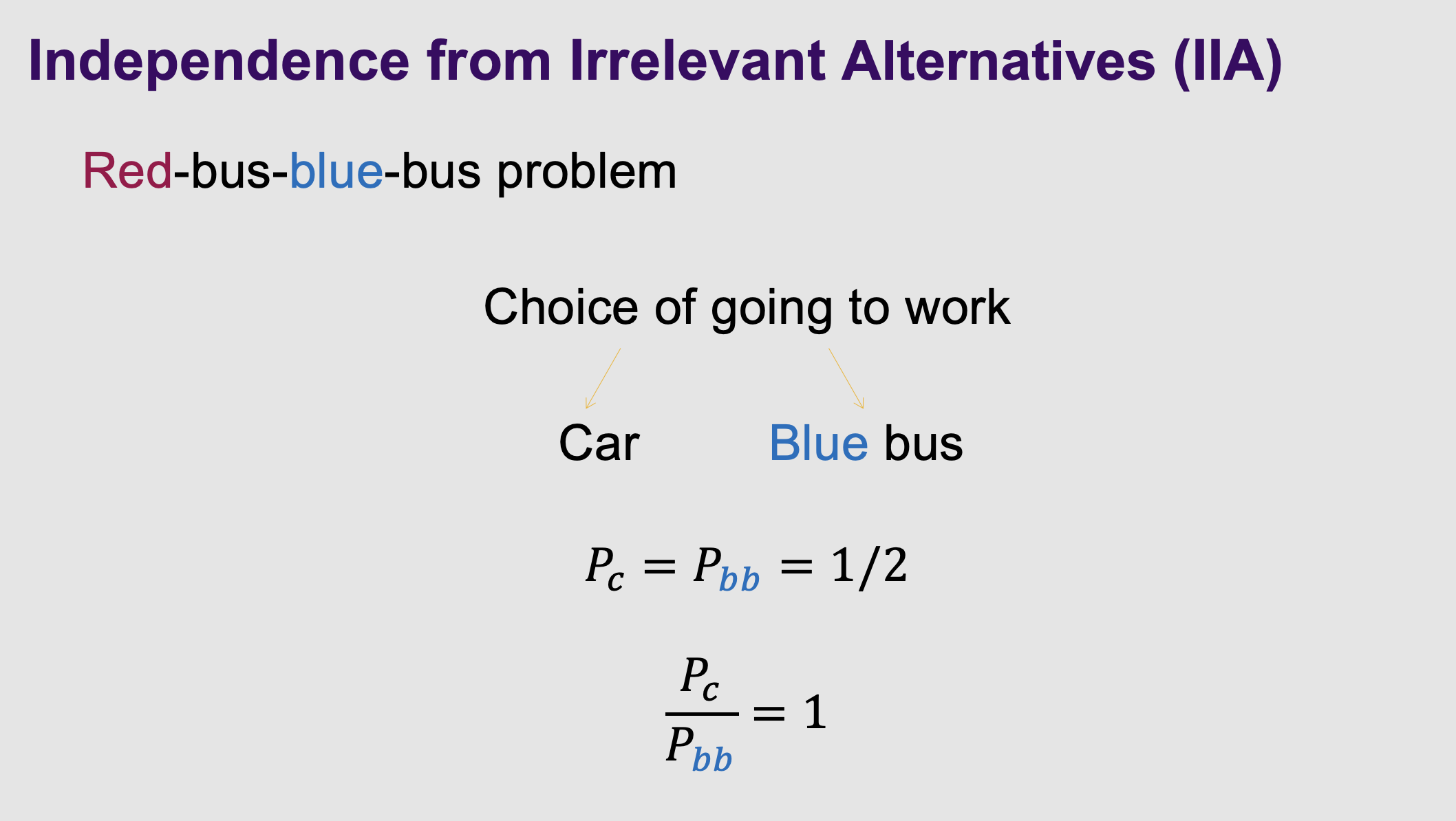
To prove why IIA is a terrible assumption, the professor introduces a famous thought experiment .

• Imagine a city where commuters have exactly two choices to get to work: driving a Car or taking a Blue Bus .

• People are evenly split. The probability of driving a Car is 50% ($1/2$), and the probability of taking the Blue Bus is 50% ($1/2$).

• Because they are equal, the ratio of Car drivers to Blue Bus riders is exactly 1 ($0.50 / 0.50 = 1$).

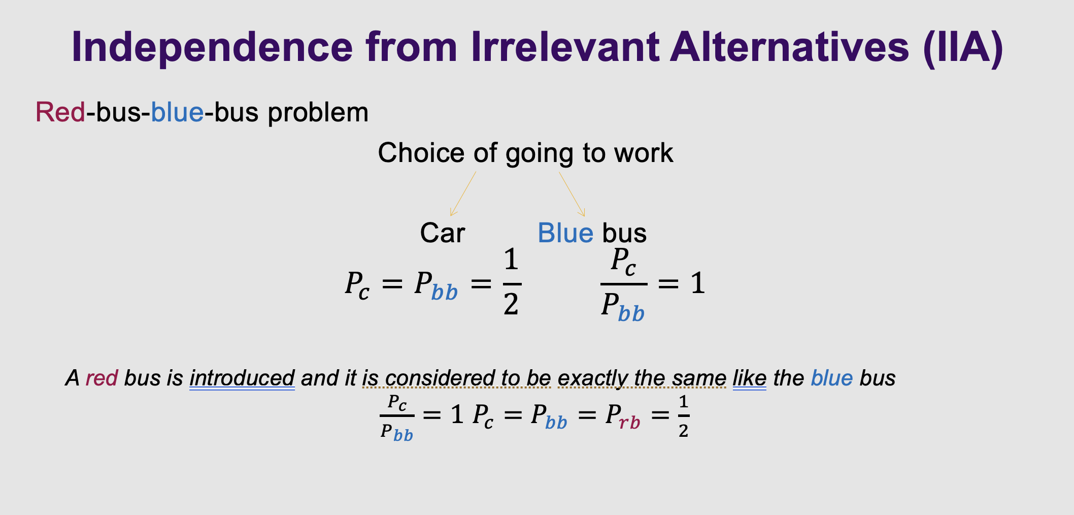
What is the second half of the problem

• Now, the city introduces a Red Bus. It is physically identical to the Blue Bus in every single way; it is just painted red.

• The MNL Math: Because of the IIA rule, the computer demands that the ratio of Car to Blue Bus must stay 1. And since the Red Bus is identical to the Blue Bus, their ratio must also be 1.

• To make all three ratios equal 1, and still sum to 100%, the computer forces them all to be exactly 33.3% ($1/3$).

• The Reality: This is completely illogical! A Car driver isn't going to stop driving just because a bus changed colors. In the real world, the Car should stay at 50%, and the two identical buses should split the transit riders (25% Blue, 25% Red). The standard MNL model fails when options are similar substitutes.

What is nested logit model

To fix the IIA problem, economists upgraded the math to create the Nested Logit Model.

• This model "partially relaxes" the IIA assumption.

• It does this by allowing the computer to recognize that some options are correlated substitutes for each other (like the Red and Blue buses) .

What is the outcome of the nested model, when we remove the auto alone

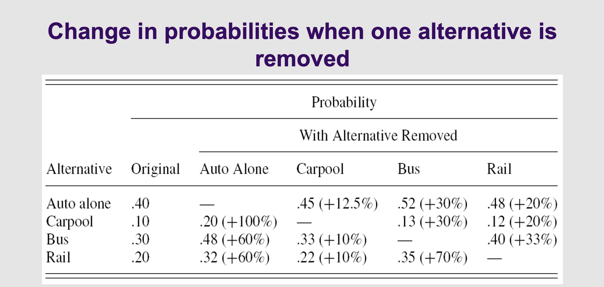
Proof that the Fix Works (The Substitution Table) This table proves the new Nested model can handle real-world behavior . Look at the "Original" column: the market is split between Auto alone (40%), Carpool (10%), Bus (30%), and Rail (20%).

Now, read the columns to see what happens when you remove an option:

• Column 1 (Remove "Auto Alone"): If driving alone is banned, where do those 40% of people go? Carpool shoots up by 100% (from 10% to 20%). Bus and Rail only go up by 60%. Logic: Stranded drivers prefer to find a ride-share rather than take the bus.

• Column 3 (Remove "Bus"): If the buses stop running, where do those 30% of people go? Rail shoots up by 70%. The car options only go up by 30%. Logic: Stranded transit riders prefer to take the train rather than buy a car.

• The Takeaway: The Nested Logit model successfully groups people into "nests." When an option is removed, people substitute within their nest first, rather than spreading out evenly.

How can we tell what are subsitutes

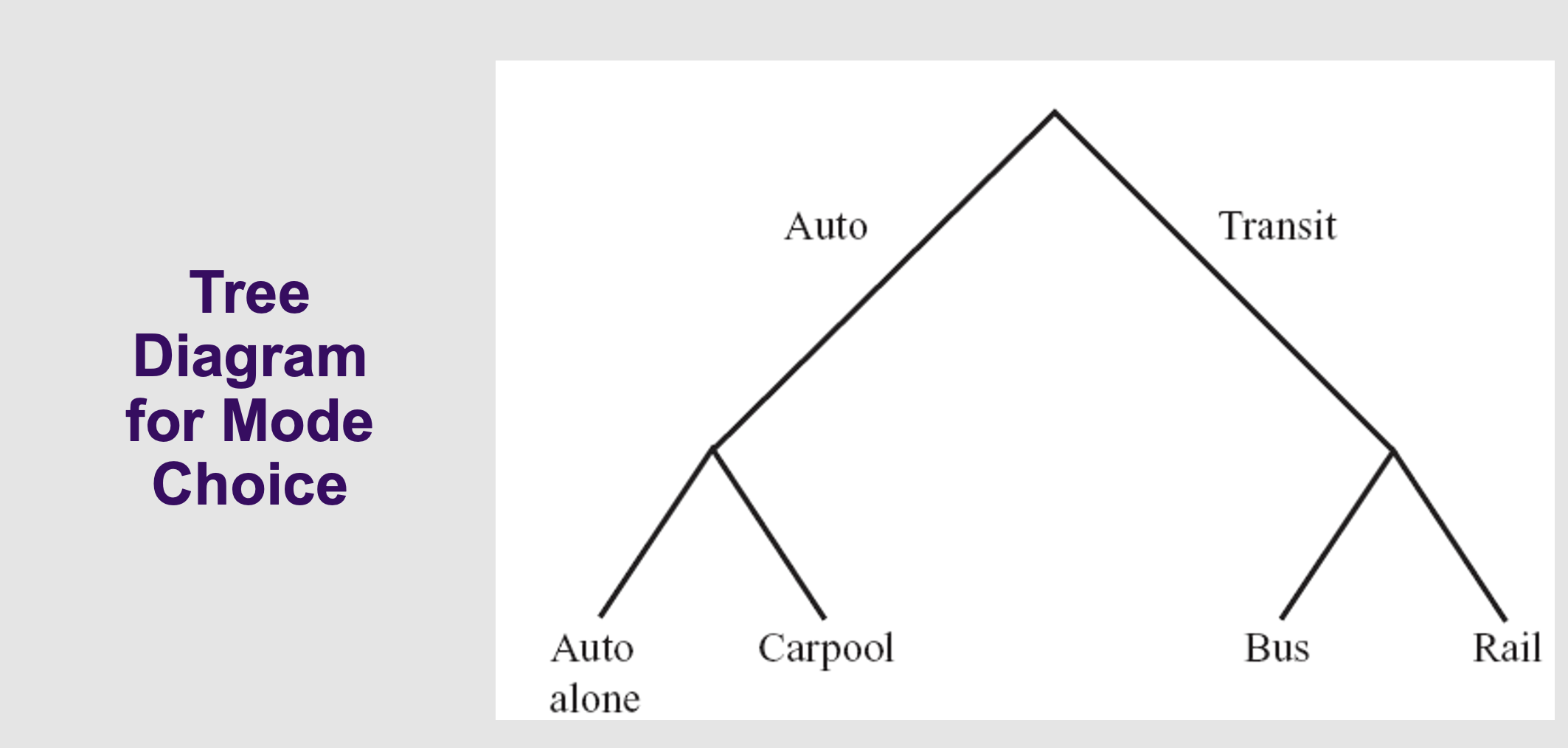
How does the computer know what substitutes with what? You draw a "Tree" for it .

• Look at Slide 29. Instead of choosing between 4 equal things, the commuter first chooses a branch: "Auto" or "Transit" . Then, they choose their specific mode inside that branch .

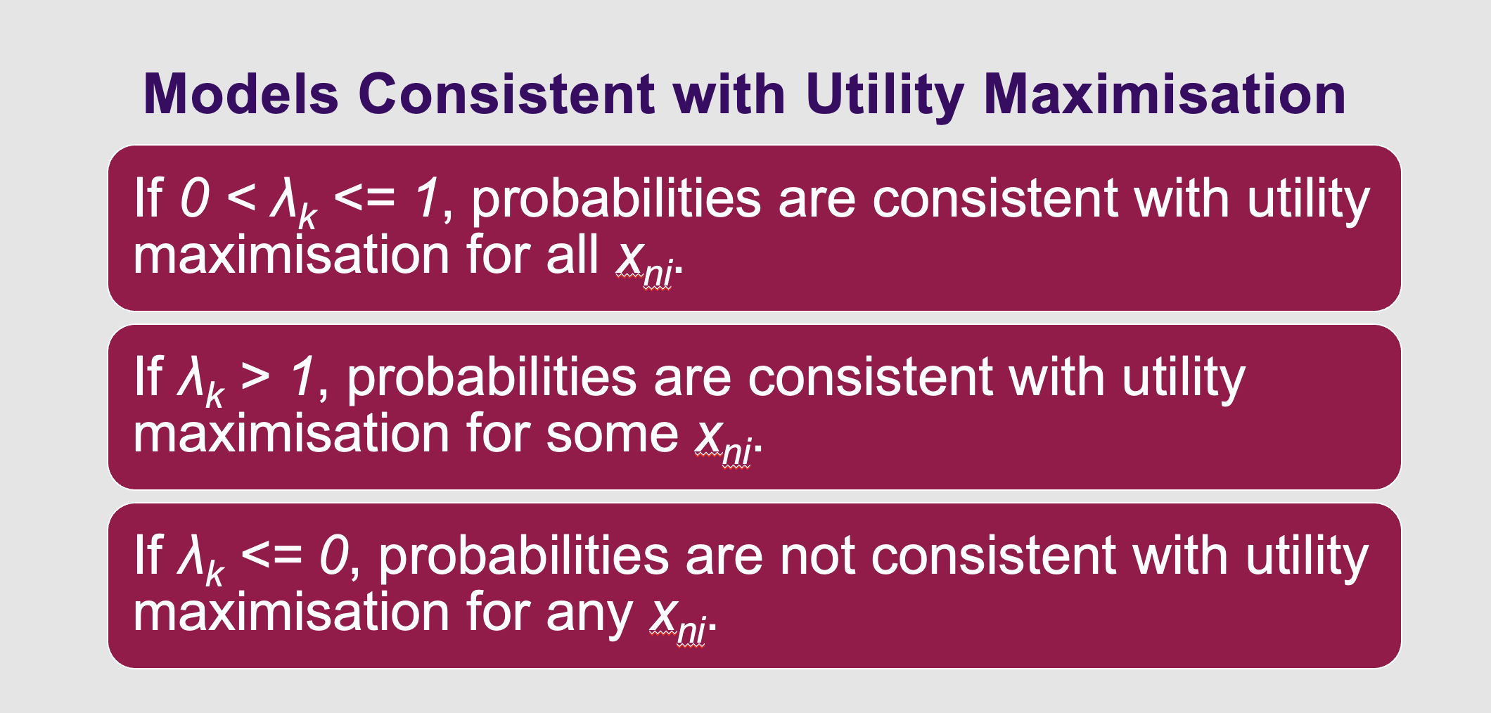
What is the golden rule for nest models

This slide tells you if your tree actually works mathematically .

• If $\lambda_k$ is between 0 and 1, the model is mathematically healthy. The computer recognizes the items in the nest are substitutes and fixes the IIA problem.

• If $\lambda_k$ equals 1, the items are completely independent. The nest effectively vanishes, and you fall right back into the flawed, basic MNL model.