Biogeography

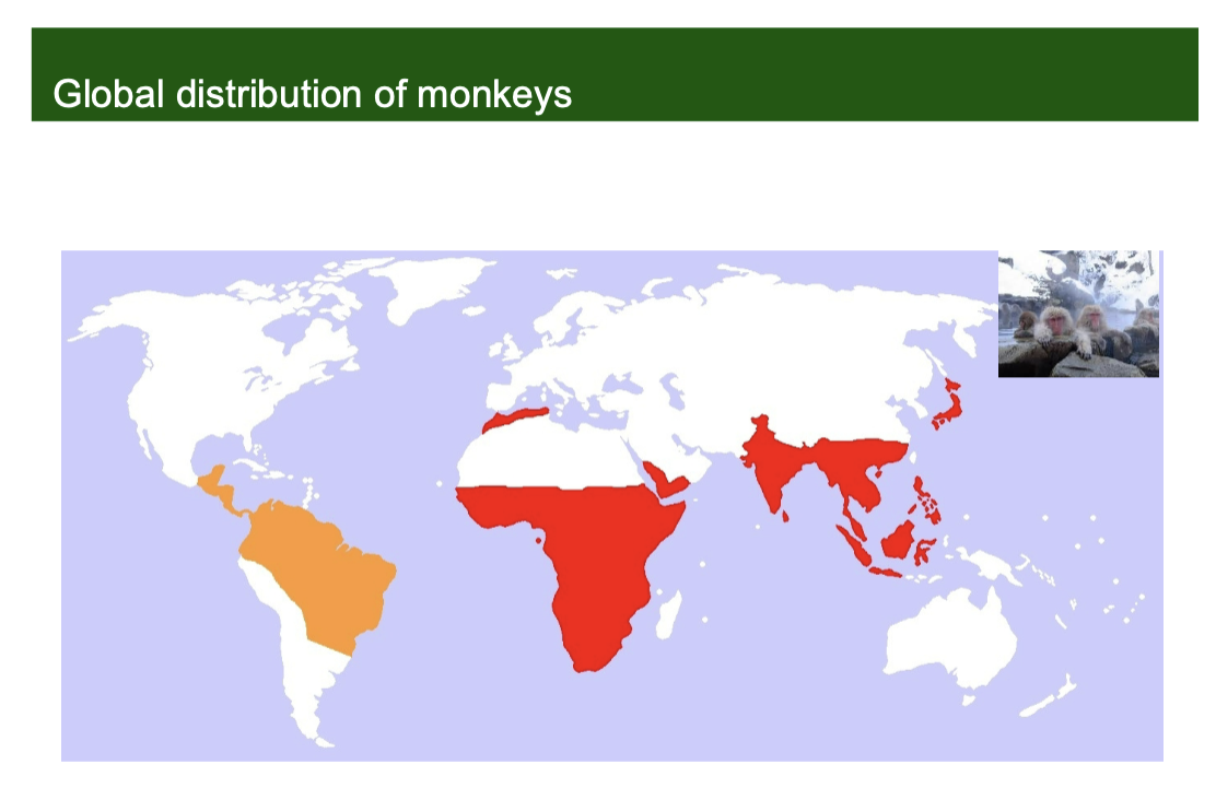
Global distribution of monkeys

Shows a map of monkey distributions, highlighting their presence in Central/South America (orange) and Africa/Asia (red)

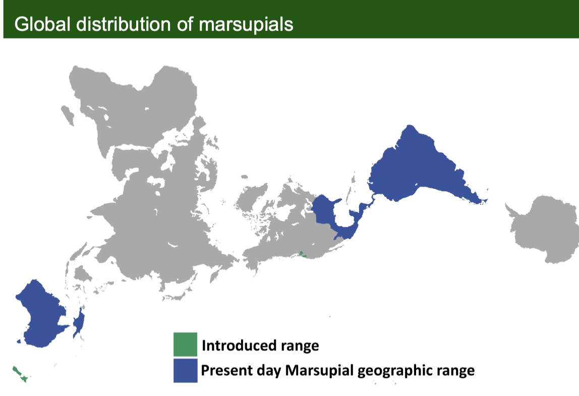
Global distribution of marsupials

Displays the present-day geographic range of marsupials, primarily in Australia and South America, as well as introduced ranges

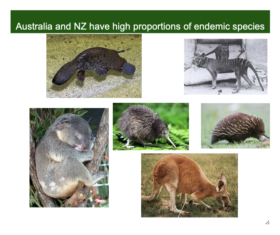
Endemic species in Australia and New Zealand

These regions have high proportions of endemic species (species found nowhere else).

Echidna, koala, kangaroo, platypus, thylacine, and kiwi

“Biodiversity” hotspots

Introduces areas with exceptionally high species richness and endemism.

One hectare of rainforest in the Amazon contains more plant species than all of Europe.

The number of fish species in the Amazon River exceeds the total number found in the entire Atlantic Ocean.

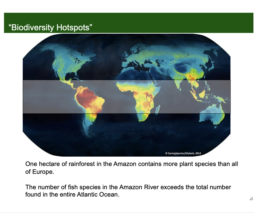
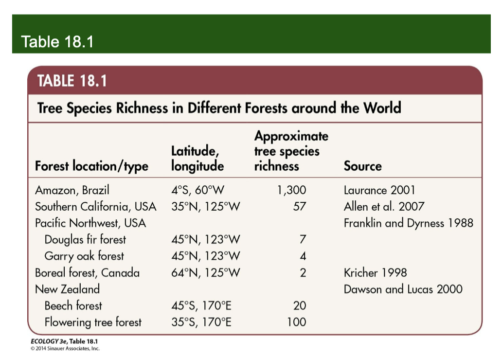
Table 18.1 - Tree Species Richness

Shows tree richness gradients: Amazon (1,300 species) vs. Boreal forest (2 species).

Biogeography

Biogeography is the study of species composition and diversity across geographic locations.

Interconnected Spatial Scales

Shows how diversity patterns are hierarchical; larger scales set the conditions for smaller ones

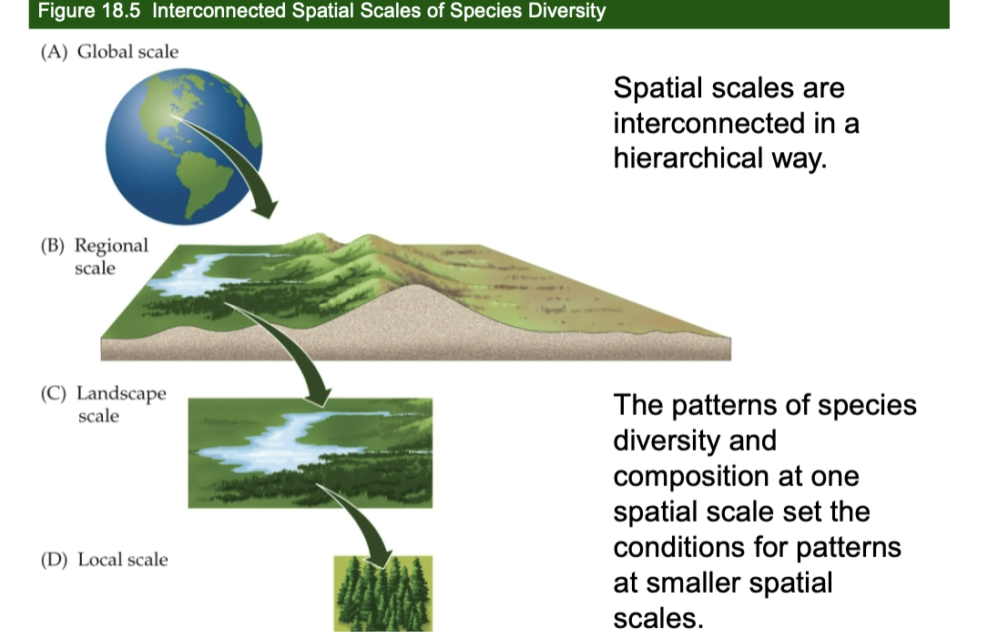
Global Scale

Encompasses the entire world

Isolation over long distances and periods (continents/oceans) influences diversity

Rates of speciation, extinction, and dispersal are the primary drivers

Regional scale

Areas with uniform climate; the species are tied to that region by dispersal limitations

Regional species pool - all the species contained within a region

Landscape Scale

Focuses on the topographic and environmental features of a region

The landscape shapes rates of migration and extinction

Local scale

Equivalent to a community

Species physiology and interactions with other species are important factors in the resulting species diversity

Variability of Scale

The actual area of a "scale" depends on the species; local scale for plants might be 10²–10^4 m², while for bacteria it might be 10² cm²

Alpha, Beta, and Gamma Diversity

Gamma: species diversity within a region (regional)

Alpha: local species diversity

Beta: the change in species composition (turnover) from one community to another, connecting local and regional scales

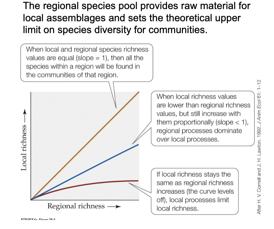
Determining Local Species Richness

The regional species pool sets the theoretical upper limit on local diversity

If the slope=1, all regional species are found locally. If the curve levels off, local processes (like competition) limit richness.

Marine Invertebrate Communities

Suggests that some communities may be limited by regional processes rather than local ones

What influences global diversity

Influenced by geographic area, isolation, evolutionary history, and climate

Alfred Russel Wallace

Known as the father of biogeography; he divided the world into six biogeographic regions

Latitudinal Gradient

Clear gradient where species diversity generally increases towards the equator

Continental Drift

Figures showing how the movement of tectonic plates over geologic time changed the positions of continents and oceans

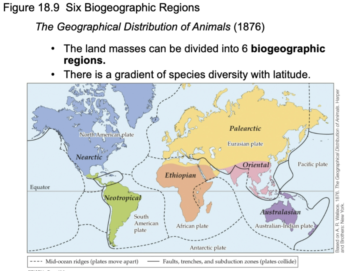
Figure 18.9

Map of the six biogeographic regions.

Regional Isolation

Neotropical, Ethiopian, and Australian regions have been isolated longest, leading to unique life. North and South America were isolated until ~6 million years ago.

Vicariance

The evolutionary separation of species by physical barriers like continental drift

Marine Biogeography

Challenges include water depth and lack of knowledge of deep oceans

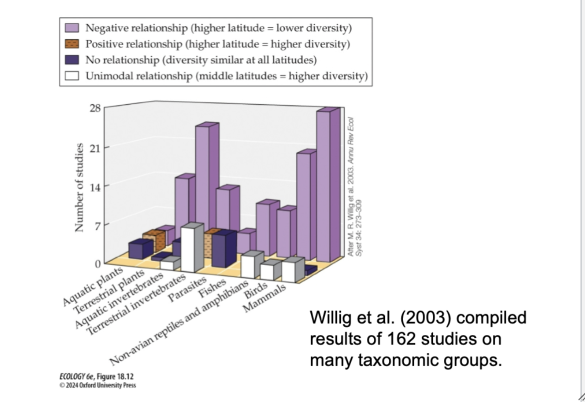
Confirming the gradient

Willig and colleagues (2003) tallied the results of 162 studies on a variety of taxonomic groups extending over broad spatial scales (20° latitude or more)

Considered whether diversity and latitude showed a negative relationship (with diversity decreasing toward the poles), a positive relationship (increasing toward the poles), a unimodal relationship (increasing toward mid-latitudes and then declining toward the poles), or no relationship.

Negative relationships were by far the most common.

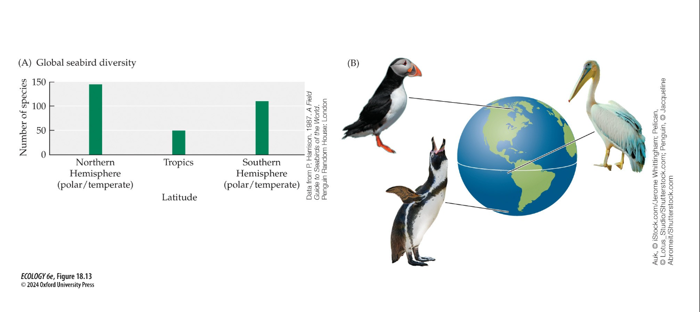
Seabird exceptions

Seabirds defy the latitudinal gradient, often showing higher richness at higher latitude and NOT AT TROPICAL CLIMATES.

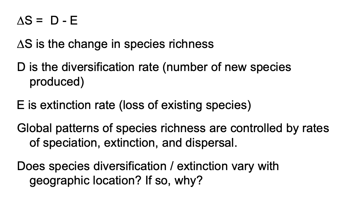
Global Richness Equations

ΔS=D−E (Change in richness = Diversification/Speciation - Extinction

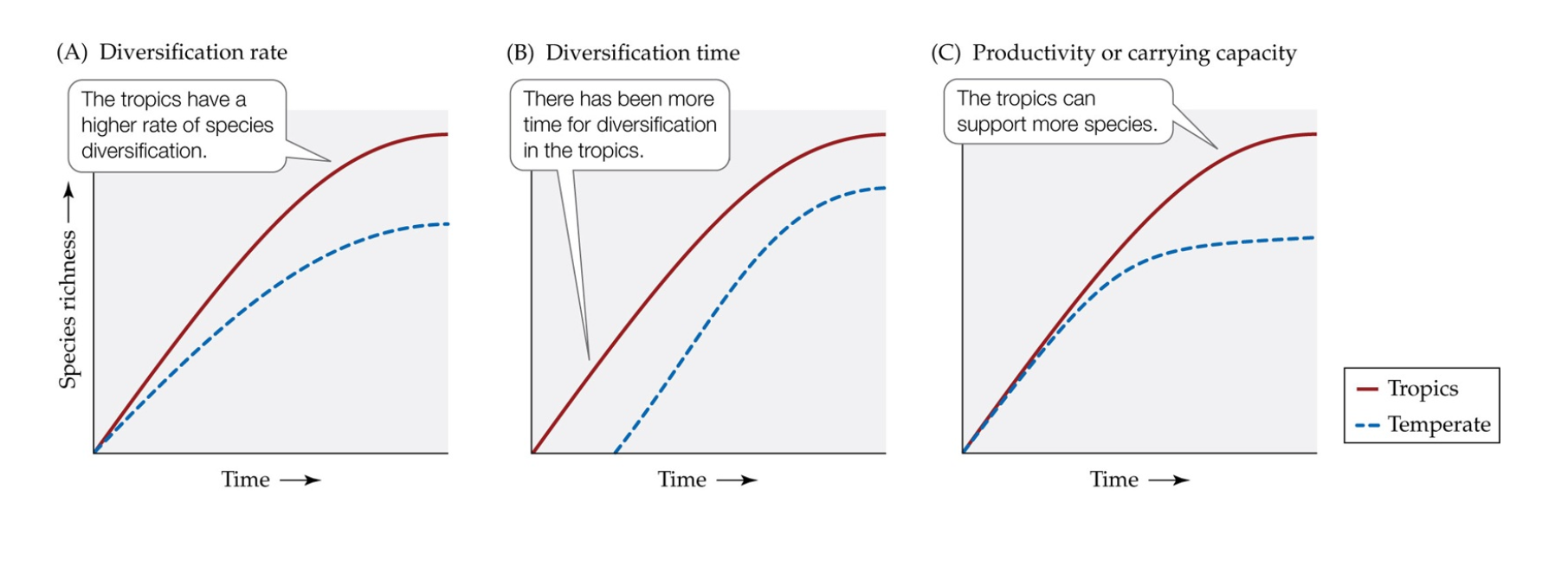
Explain the Latitudinal Gradient in Species Richness

Proposes Speciation Rate, Speciation Time, and Productivity as drivers for the latitudinal gradient

Species Diversification Rate

Tropics have the largest, most thermally stable land area, likely decreasing extinction and increasing speciation by isolation.

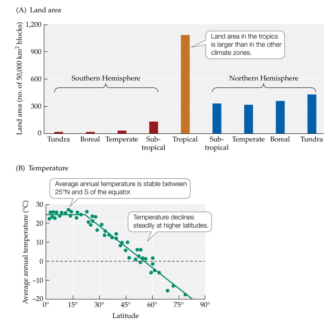
Land and Temperature Influencing Species Diversity?

Michael Rosenzweig hypothesized that two characteristics of the tropics lead to high speciation rates and low extinction rates: (A) their land area and (B) their stable temperature

Species Diversification Time

Tropics were climatically stable longer, allowing more time for evolution

Tropics as Source

Most species originate in the tropics and spread toward the poles; the tropics act as a "cradle" and a "museum"

Cradle - species originate in there and to other regions, primary source of new species

Museum - safe havens where older species persist

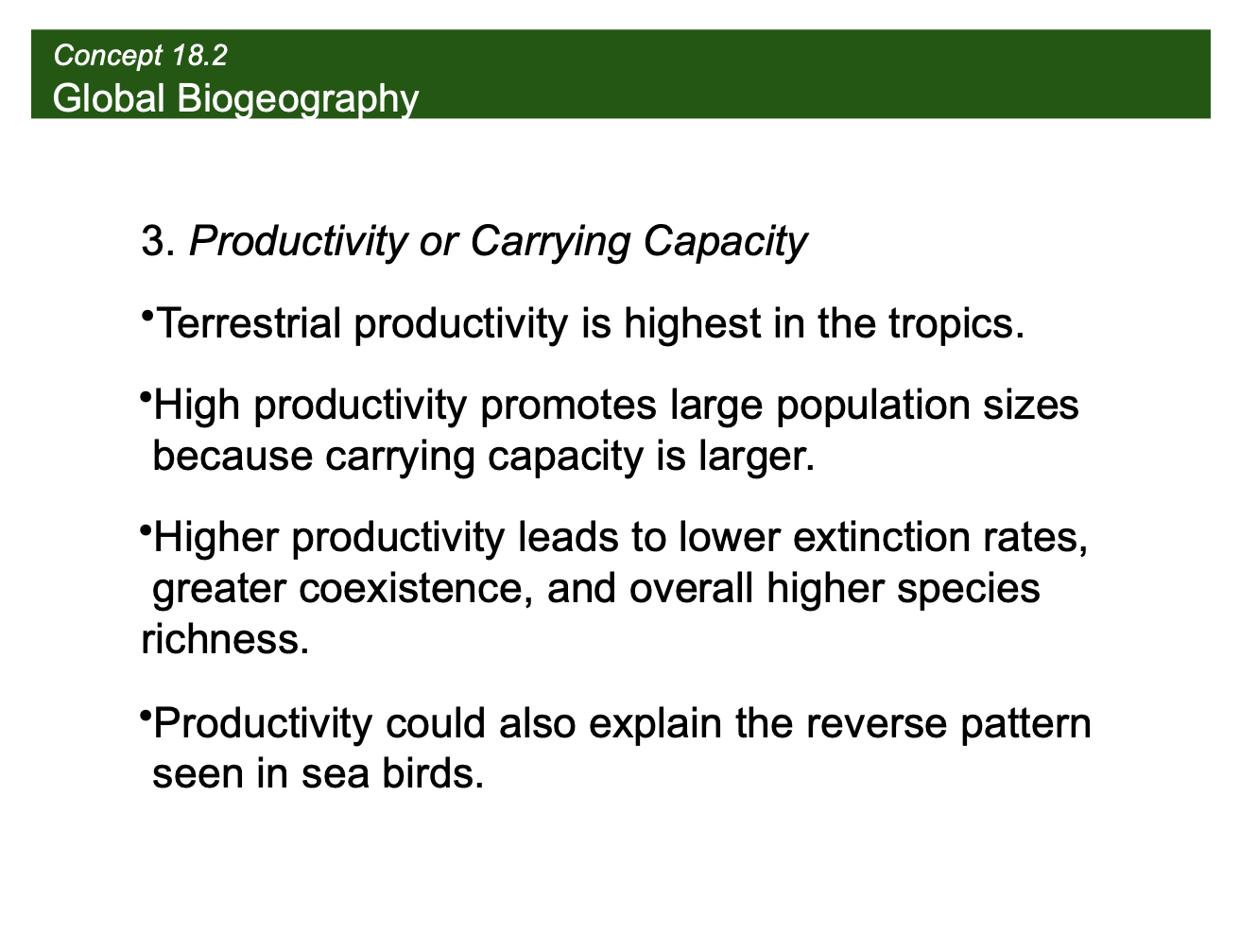
Productivity/Carrying Capacity

High tropical productivity supports larger populations, higher carrying capacity, and lower extinction rates

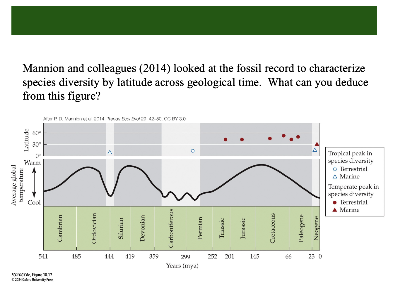
Fossil records

Shows that tropical diversity has been higher for most of Earth's history.

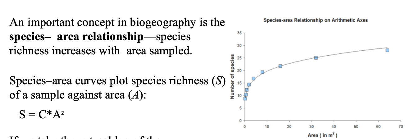
Species-Area Relationship

Formula: S=cA^z. As area (A) increases, species richness (S) increases

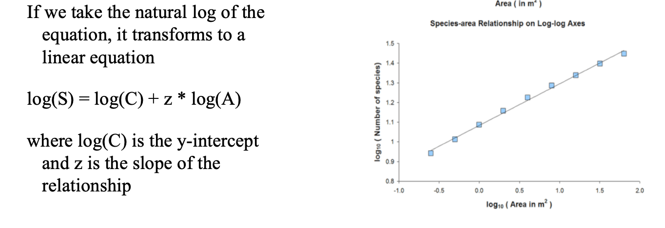
Log Transformation

Shows how scientists turn the curve into a straight line (logS=logc+zlogA) to calculate the slope (z).

HC Watson

Plotted first species-area relationship, using plants in the Great Britain…in 1859

Islands as Models

"Islands" aren't just in the ocean; they can be mountaintops or forest fragments.

Big islands vs small islands

Data showing that big islands have more species than small ones, and near islands have more than far ones

Equilibrium Theory

MacArthur and Wilson’s idea: Species number is a balance between Immigration and Extinction

Proves that as island size increases 10x, species count doubles

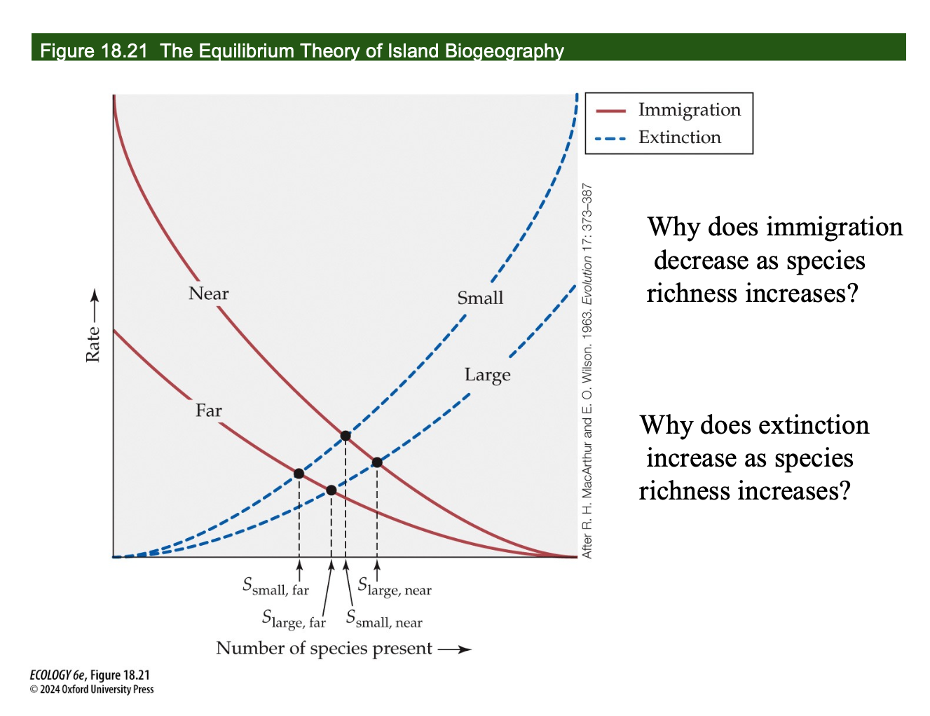
The Equilibrium Graph

dCrucial graph showing where Immigration and Extinction curves cross.

According to the Equilibrium Theory of Island Biogeography, the rate of immigration decreases as the number of species on an island increases for two primary reasons:

Fewer "New" Species: As more species become established on an island, the likelihood that a newly arriving individual belongs to a species that is not already present decreases. Eventually, every individual that arrives will belong to a species that is already a resident, bringing the immigration rate of "new" species to zero.

Reduced Opportunities for Successful Colonization: As species richness increases, competition for limited resources also increases. Incoming individuals find it more difficult to establish themselves in a community that is already crowded and biologically divers

Krakatau

A real-world test: Life returned to a volcanic island and reached a stable equilibrium of ~30 bird species

To test their theory, MacArthur and Wilson used

Krakatau as an example, and island that had a

violent volcanic explosion that killed everything on

the island.

Based on immigration and extinction rates from

multiple surveys, they predicted that the islands

could support ~ 30 bird species, with a predicted

turnover of 1 species per year

Mangrove Experiment

Simberloff & Wilson killed all insects on mangrove islands with insecticide to watch them recolonize.

Mainland vs. Island

Mainlands have higher immigration and lower extinction because there are no water barriers.

The Rescue Effect

Species on mainlands are less likely to go extinct because new individuals from nearby populations "rescue" them.

Habitat Fragmentation

A closing look at how human-caused "islands" in the Amazon impact biodiversity.