Y2 - Intermediate Macroeconomics S2 Notes

Phillips Curve in the Barro and Gordon (1983) Discretion Model:

Phillips Curve Relation: U = Uⁿ - α(π - πᵉ)

• U = natural UN; π= πᵉ means realised inflation = Exp INF πᵉ (when policymaker has perfect control)

• based on private sector knowledge of policymaker objectives and economy structure

• α = weighting parameter, measures deviation of πᵉ from π impacting whether Uⁿ is higher or lower than U; affects slope of Phillips Curve ****.

Loss function in the Barro and Gordon (1983) Discretion Model: .

Loss function: L = L(U,π) = U+γπ², 0 ≤ γ ≤ ∞

• measures amount of disutility felt by monetary authorities

• Higher L = Higher disutility

• Assumes U = UN, larger values yield increasing disutility

• Deviations π from zero increase, so does disutility

• γ (gamma) = denotes weight attached to π² relative to U

• Suggests BoE has 0% π target as inflation would not impact L

• if γ = 0 , Loss function is L = L(U,π) = U evidently..

Finding optimal rate of inflation to set by differentiation, as part of Barro and Gordon Discretion Game:

Step (4): Substitute Phillips Curve into Loss function

L = U+γπ² U = Uⁿ - α(π - πᵉ)

L = Uⁿ - α(π - πᵉ)+γπ²

Step (5 and 6) Find π that is optimal to set, diff L w.r. to π and solve for π

dL / dπ = -α+2γπ = 0

• explanation: Uⁿ is void ; (π - πᵉ) is removed to leave -α ; γπ² —> power drop down and multiplied

Solving for π yields: π = α / 2γ

• put π LHS and α RHS and place

Optimal for policymaker to set +π, inflation bias

Finding optimal level of unemployment via substitution, as part of Barro and Gordon Discretion Game:

Step (7): Expected inflation = realised inflation and prove by subbing in πᵉ and π into original Phillips Curve equation (8,9)

<aside> 💡

E [π] = πᵉ = α / 2γ

• U = natural rate.

U = Uⁿ - α(π - πᵉ)

= **Uⁿ - α (α / 2γ -  α / 2γ)** 

= **Uⁿ** 

</aside>.

Loss discretion in the Barro and Gordon Discretion Game:

L = U + γπ²

= Uⁿ + (α / 2γ)^2, sometimes called ‘discretionary policy’

Loss discretion if the PM was able to commit to zero inflation (backed by private sector) in the as part of Barro and Gordon Discretion Game:

π = 0, πᵉ = 0 , U = Uⁿ

• U = Uⁿ because.. Uⁿ - α(0-0)

Losses: = L = Uⁿ + γ [0]^2 = Uⁿ

Comparing losses in Baron and Gordon’s model (rule vs discretion):

Comparing losses:

• Rule: L = Uⁿ (preferred as its smaller)

• Discretion: L = Uⁿ + α^2 / 4γ

PM announces a rule of zero inflation, belueved by PS, temptation to cheat to reduce U below Uⁿ in the Baron and Gordon rule vs discretion model:

through setting positive π of α / 2γ

<aside> 💡

U = Uⁿ - α(π - πᵉ)

= Uⁿ - α (α / 2γ - 0) = Uⁿ - (α^2 / 2γ)

Losses:= Uⁿ - (α^2 / 2γ) + γ [α / 2γ)^2

= Uⁿ - α^2 / 2γ + α^2 / 4γ**

= Uⁿ - α^2 / 4γ**

</aside>

Step (17): Consequences if PM adhered to its promise if the private sector set πᵉ = a / 2γ in the Baron and Gordon rule vs discretion model:

U = Uⁿ - α(π - πᵉ)

= Uⁿ - α(0 - α^2 / 2γ)
= Uⁿ + α^2 / 2γ

L = Uⁿ + α^2 / 2γ + γ(0)^2 = Uⁿ + α^2 / 2γ

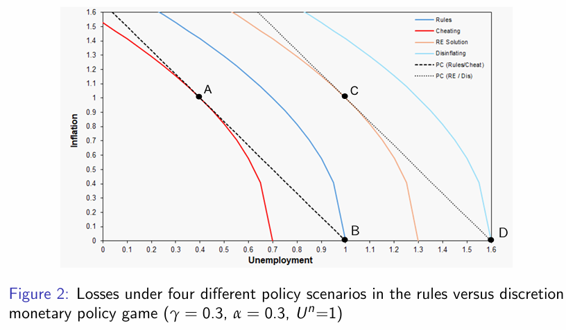
Comparing losses for policymakers n the Baron and Gordon rule vs discretion model comparing cheating, discretion and disinflation:

L^Rule = Uⁿ

L^Discretion = Uⁿ+ α^2 / 4γ

L^Cheat = Uⁿ - α^2 / 4γ

L^Disinflation = Uⁿ _ α^2 / 2γ

L^Cheat < L^Rule < L^Discretion < L^Disinflation.

Point A: This is the solution for cheating. Point B: This is the solution under a rule. Point C: This is the solution under discretion (sometimes called the rational expectations (RE) solution ). Point D: This is the solution under disin ation (worst case scenario).

Baron and Gordon model solutions to cheating:

Solution: Commitment technology, allowing policymakers to abide by their promises and adhere to binding rules

• granting greater levels of central bank independence

  • politicians cannot interfere with policy-making decisions

Partisan Politics and developments:

Partisan Politics: Left-wing parties prefer combinations of Q and UN, differing systematically from those chosen by RW parties (Hibbs, 1977)

• Left-wing parties are assumed to be more willing to bear costs of INF —> lower UN and increase EG

• incorporates exploitable trade-offs between INF and UN via assumption of adaptive expectations

  • developments in 1960s suggest a trade-off is not easily exploitable

Rational Partisan Theory (Alesina and Rosenthal, 2004) and author inputs:

• Similar model, within a rational expectations framework

• (Nordhaus 1975) predicts EG should be higher before administration comes to power, irrespective of political ideology

• (Tufte, 1978) argues for EG manipulation to engineer an economic boom before an election

  • e.g. 3rd year US economic boom before inflation year

• Business Cycle occurs due to uncertainty generated by competitive partisan politics

Establishing structure of economy and assumptions within Rational Partisan Theory:

Step (1) structure of economy

y =γ (πt - wt)+ ȳ

yt = GDP growth rate, πt = inflation, wt = growth rate of nominal wages, ȳ = natural rate of EG, γ > 0 as a parameter, t = time subscript

Step (2) we assume nominal growth in wages, wt = πᵉ

πᵉ = Inflation rate expected at start of period t

Expression: y =γ(πt -πᵉ )+ȳ

Model envisages party D (democratic) and party P (Republican)

• D is more concerned with growth and UN, less with inflation

• Preferences between parties differ, captured by different objective functions

Rational Partisan Theory Party D policy preferences:

uD = - (πt / πˉD)^2 + bD*yt (higher Y increaes utility)

• deviations from πˉD lower utility

such that πˉD > 0 and bD > 0

πˉD = target INF rate associated with Party D

bD = extent to which D cares about output

Rational Partisan Theory Party R policy preferences:

uR = - (πt / πˉR)^2 + bR*yt (higher Y increaes utility)

• deviations from πˉR lower utility

• such that πˉR > 0 and bR > 0

Policymaker R benefits from an unexpected burst of inflation when substituting γ(πt -πᵉ )+ȳ into the objective function

Rational Partisan Theory assumptions of inflation and output growth tolerance:

Step (11) Assumptions of inflation tolerance

πˉD > πˉR > 0; Party D has a higher tolerance of inflation

Step (12) Assumption of output growth importance

bD > bR > 0 ; Party D cares more for output growth relative to inflation

</aside>

Voter preferences of Rational Partisan Theory:

Voter (i)’s preferences:

• Voters face electoral uncertainty, so inflation expectations are a probability-weighted average of both party’s inflation policies

ui = - (πt - πˉi)^2 + biγ (πt - πᵉ) + biyˉ

• Voter i benefits from an unexpected burst of inflation

Timing of events of Rational Partisan Theory:

• Wage contracts are signed before the election, based on expected π

• Elections occur and winning party is chosen

• Policymaker chooses inflation for the period

πt = πD* = πD +bDγ / 2 ; πe.t.= πD =πˉD +bDγ / 2 ; yt = yˉ

• party R’s optimal policy, πD >πR

• Output occurs, driven by inflation gaps

• New wage contracts are signed for next period

• Incumbent policymaker sets inflation again with no electoral uncertainty

• Natural level of output and expectations fully adjusted

Electoral uncertainty and inflation of Rational Partisan Theory:

• Election outcomes are uncertain, so voters assign probability P that party D wins + (1-P) that party R wins

• Before election (P1), Eπ = weighted average of both party inflation targets

  • π1e = PπD+(1−P) πR

• Party D wins: Actual π > Eπ —> positive surprise inflation —> Q rises above natural level

• Party R wins: Actual π < Eπ —> negative surprise inflation —> Q falls below natural level

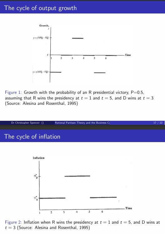
Recessionary impact of electoral uncertainty in Rational Partisan Theory:

• Degree of surprise impacts amplitude of output fluctuations

  • as P increases, the greater the recession is generated by R victory, because the less expected is the inflation shock

  • R (prob of D winning) causes recessions if they win because of high expectations of D victory

    • Period 1 downturn is necessary to eradicate inflationary expectations from public

Conventional policy limits of QE:

Conventional policy limits

• Nominal IR are typically not negative

• Zero Lower bound for Nominal IR limits extent to which conventional MP can be used to stimulate demand in recession

• QE - unconventional monetary policy as a last resort

“The problem with QE is that it works in practice, but it doesn’t work in theory” (Ben Bernanke, January 2014)

QE explained + comparison to OMO:

Quantitative Easing

• CB creates electronic accounts credited with new cash balance —> purchase assets from financial institutions —> increases private sector (commercial bank) cash balance

• Modern EQIV of printing but the policy is unwound

• CB acquires assets in the process

• Adopted by Bank of Japan in early 2000s, BoE in 2009

QE is financed by newly created money, expanding CB balance sheet.

Conventional OMO’s swap assets without changing balance sheet size

Purchasing bonds is risky because of loss of value, but QE is riskier as it entails balance sheet expansion.

Treasury approval of QE:

• Bank’s ability to make asset purchases requires approval

• The use of QE is effectively at the discretion of government, undermining operational independence

  • without indemnity the Bank could be exposed to capital looses —> must offset by varying balance sheet size and income earned from assets

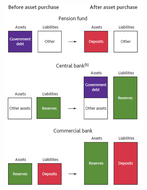
How does EQ work in practice

• The Bank of England buys £1bn of government bonds.

• It creates electronic money

• If bought from a pension fund (non-bank):

  • The pension fund’s bank credits its deposit account.

  • The Bank credits reserves to the commercial bank.

  • Result: Reserves ↑ and private sector deposits ↑.

• If bought from a commercial bank:

  • Bonds are swapped for reserves.

  • Result: Reserves ↑ but deposits unchanged.

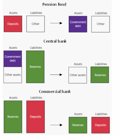
Unwinding QE:

• Unwinding by the CB selling government bonds back to non-financial institutions such as pension funds —> CB balance sheet shrinks

  • NFI replace deposits with cash + BoE holds cash

• Commercial bank liabilities fall, but has assets in form of CB reserves

Features of QE including rebalancing portfolios, targets and shadow banking:

• Asset purchases operate to a quantitative target

• Scale and scope of QE operations differ across central banks

• QE leaves private investors long in cash that yields a low return

  • investors rebalance portfolios towards assets such as corporate bonds

    • private assets = central elements of shadow banking system

    • Drives up prices for corporate bonds and equities, depressing IR paid in shadow banking sector

      • Lower financing costs in shadow banking sector—> corporations can engage in investment and hiring —> boost AD —> macro performance

• CB purchases of L-T bonds push money into areas like corporate bonds —> cheaper for corporations to borrow

QE and Credibility in Economy:

QE and Credibility

• QE can signal that BoE will keep IR low for time —> boosts C, Inv and AD

  • promising low rates whilst tolerating high INF may lack credibility (time-consistency problem)

    • Rise in INF —> Bank raises IR to protect target —> Mistrust

  • bank rate rose sharply (5.25% in April 2024) —> bank begun Quantitative Tightening

    • QT reduces balance sheet and raises L-T rates, bonds may be sold at a loss

QE —> Liquidity Premia effect:

CB provides liquidity to markets at times when liquidity may not be forthcoming from other financial market participants

• Important when financial markets are dis-functional

Confidence and Bank Lending effects of QE:

Confidence effects: Consumer confidence may be boosted by improved economic outlook that actors may associate with QE

Bank Lending effect: Increased reserves in banking system —> increased commercial bank lending

• MPC did not expect significance in which macroeconomic impacts occur

Natural rate of unemployment definition and details:

Natural rate of unemployment: The average rate of unemployment around which the economy fluctuates; normal UN when there is neither a recession or boom

• Natural rate strips out fluctuations and is a much smoother line than booms or recessions

• Recession: AC UN > NAT UN and vice versa in a boom

• expected to be constant overtime, but adjusting in response to change in labour market legislation and supply side factors; expected to change very slowly overtime

Model of Natural Rate of Unemployment and Assumptions:

L = no. of workers in labor force

• L = E + U

E = no. of employed workers

U = no. of unemployed

U/L  = unemployment rate (%)

Assumptions:

• L is fixed and this exogenous

• During any given month (both exogenous):

  • S = rate of job separations: fraction of employed workers that become separated from their jobs

  • f = rate of job finding: fraction of unemployed workers that find jobs

  • both are bound from 0-1; if 1% of the employed lose their jobs each month, the rate job separation rate will be s=0.01; if 3 percent of the unemployed find employment each month, the job finding rate will be f=0.03.

Steady-state condition definition and formulae, as well as example:

Steady-state condition:

• The labour market is in steady state, or LR EQ if the UN rate is constant

$$s <em> E = f </em> U$$

• #. of employed people who lose or leave their jobs = #. of unemployed people who find jobs

Example:

• s = 0.01, f = 0.19, find the Natural Rate of UN

U / L = s / s + f = 0.01 / 0.01 + 0.19 = 0.05 or 5%

Policy implications of Natural UN:

Policy implications of Natural UN

• A policy will reduce the Natural UN only if it lowers s or increases f

  • Therefore, if government can affect s and f, it can influence UN

Frictional Unemployment and Duration of UN:

Frictional UN: caused by the time it takes workers to search for a job

• occurs when wages are flexible and jobs are plentiful

  • workers have diff abilities, jobs have different skill requirements, non-instant geographical mobility and imperfect flow of information e.g. vacancies

• Duration:

  • most spells are short-term but most weeks of UN are attributable to a small number of L-T persons

Search and match unemployment theory:

Search and match theory:

• Unemployment arises as the result of Frictional UN and suitable matches, so that even in EQ there are simultaneously unemployed workers and unfilled vacancies

• Workers may be overqualified or underqualified, constituting a misallocation of labour resources

  • solution: free movement in EU or web-based job sites

Sectoral shifts as part of Structural issues, backed up with stats:

Structural issues:

• Sectoral shifts:

  • e.g. coal mining communities in the North of England impacted by closure of mines and collieries, despite being skilled at mining

  • e.g. decline of manufacturing and rise in service industries (81% total UK economic output in 2018)

  • UK employment stats:

    • 1980: 59.8% agriculture, 37.6% industry, 2.6% services

    • 2001: 2% agriculture, 25% industry, 73% services

  • Examples:

    • Industrial Revolution (1800s): agricultural decline and manufacturing soaring

    • Energy Crisis (1970s): demand shifts from larger —> smaller cars

  • Small sectoral shifts occur in our dynamic economy, contributing to Frictional UN

Unemployment Insurance (UI):

Unemployment Insurance (UI):

• UI pays part of a worker’s former wages for a limited time after a job loss

• UI increases search unemployment as it reduces:

  • Unemployed Opp Cost

  • Urgency of finding work

  • f = fraction of unemployed workers that find jobs

• Benefits: better matches, greater productivity, higher incomes, less financial pressure

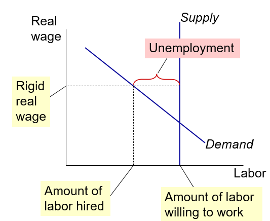
Unemployment from Real-Wage Rigidity:

• If real wage is stuck about EQ, there are insufficient jobs

  • Amount of labour demanded by firms > amount of labour willing to work —> Structural UN

• Wages are not always flexible, so real wage can be stuck at market clearing level

• Jobs are rationed and not all individuals are willing; too many people chasing too few jobs

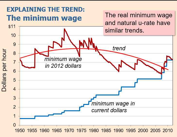
Reasons for Wage-Rigidity: Minimum wage laws:

Reasons for Wage-Rigidity

• Minimum wage laws:

  • Min wage > EQ wage of unskilled workers

    • Study: 10% increase in Min Wage reduces teen employment by 1-3%

  • Evaluation: Min wage cannot explain most of Natural UN as most wages are above Min wage

Reasons for Wage-Rigidity: Labour Unions:

• Unions exercise monopoly power —> secure higher wages

• Union wage > EQ wage —> Unemployment

  • Insiders: Employed Union Workers whose interest is to keep wages high

  • Outsiders: Unemployed Non-Union workers who prefer EQ, so there are enough jobs

• Union membership in UK:

  • 1980: 50% —> 2000: 28%

Reasons for Wage-Rigidity: Efficiency Wages:

• Efficiency wages:

  • Theories in which higher wages increase worker productivity by:

    • attracting higher quality job applicants

    • Increasing worker effort

    • reducing turnover, costly to firms

    • improving health of workers

  • Firms willingly pay above-EQ wages to raise productivity —> Structural UN

Solow Model (1956)

• The closed economy Solow model of LREQ

  • How a country’s standard of living depends on its respective rates of saving, population, growth and technological progress

  • Notion of a steady state, capturing economic growth along a balanced growth path

The Solow Model (1956)

• The workhorse model of LR economic Growth

• Dynamic model involving variables changing overtime, but is NOT a model of short-run economic fluctuations

Solow Growth Model in terms of summary, technological progress, and human capital:

• The Solow growth model is the most well-known model of long-run economic growth.

• Adding technological progress to the model allows us to account for the fact that GDP per capita is observed to grow over time.

• Although some of its predictions hold in the real world, it also has some shortcomings, some of which are not explored here.

• First, technological progress is treated as being exogenous, whereas in practice, there are compelling reasons to view such progress as being determined endogenously.

• Second, it says little about the role that human capital plays in determining growth.

• It is, however, a highly influential model that forms the basis of more recent theories which aim to address the type of shortcomings listed above

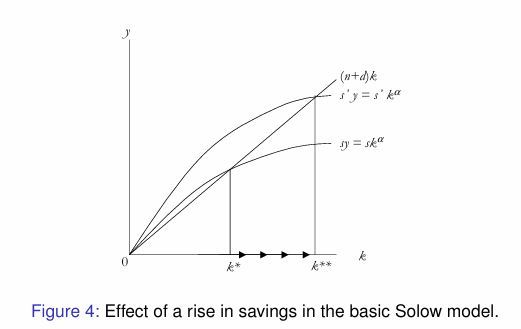
Prediction of Solow Growth Model: Rise in Savings:

• Expression (24) it is evident that the savings rate s will affect the steady state value of capital per worker, k*

• Higher s —> higher k* —> higher y*

Solow Model predicts that countries with higher rates of savings and investment —> higher levels of capital and income per worker in the LR

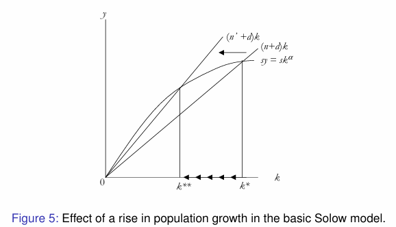
Prediction of Solow Growth Model: Rise in Populations:

• Expression (24), evident that the rate of pop growth n will affect steady state of value of capital per worker

• higher n —> lower K* —> lower y*

<aside> 💡

The Solow model predicts that countries with higher rates of population growth will have lower levels of capital and income per worker in the long run.

</aside>

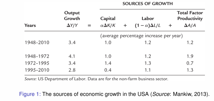
Growth Accounting:

• Productivity growth: Improvements in TFP account for a larger share in LR growth in income per capita

• Input accumulation is important but not sufficient: investment in capital explains part of growth, but independently cannot account for sustained increases in living standards

• Rapid growth often combines both: high savings and investment rates + productivity improvements help explain the growth of Western Europe and East Asia

Output growth equation:

Output growth = capital contribution + labour contribution + TFP Growth

• Fundamental EQ of growth accounting, allowing us to measure three sources of growth: changes in K, L and TFP

• TFP is the only component not directly observed

Interpreting Total Factor Productivity capturing tech change and EG:

• Captures tech change but other factors too such as:

  • Improvements in management: ability to organise work or improve management quality

  • Better allocation of resources: reallocation of production factors (labour and capital) from low-productivity sectors (e.g., agriculture) to high-productivity sectors (e.g., industry/services).

  • Institutional changes: degree of competition, legal frameworks, regulatory efficiency.

  • Measurement error: discrepancies between the recorded data and true economic values.

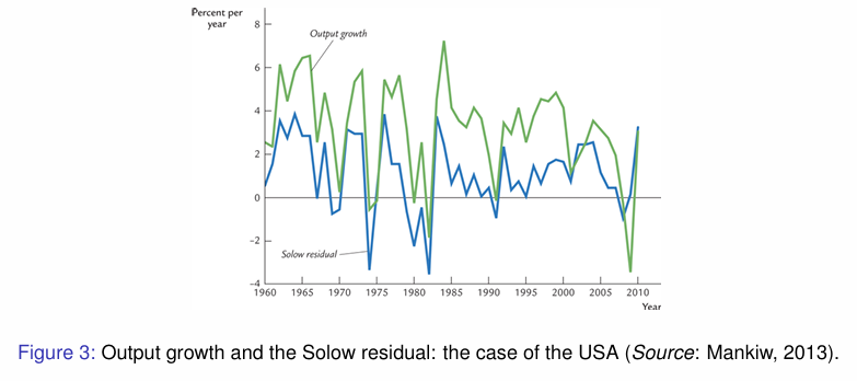
“New Economy”, linking to productivity growth, output growth and Solow Residual:

• Spread of computers and increasing use of information tech

• IT revolution explains rise in productivity growth but also slowdown after 1972

  • growth temporarily slowed during adaptation of factories to new production techniques associated with information tech and learning; widespread adoption of new tech

Solow Paradox: You can see the computer age everywhere but in the productivity statistics

• Solow intended the residual to be used to analyse LR growth

  • Prescott suggests the residual is useful in analysing tech change over shorter time periods

• Solow residual fluctuates quite markedly over the sample period 1960-2010.

• Solow residual is highly correlated with movements in output suggests that a major cause of recessions is adverse shocks to technology

  • however, many shocks cannot be precisely identified

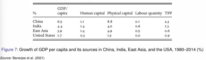
Economic growth in the West vs East and Total Factor Productivity

Economic growth in the West and Total Factor Productivity

• Fast growth in Europe and the USA in the post-WWII decades.

• Growth in GDP per capita exceeded 2.5% per year everywhere (except in the UK) aiming to be on par with USA.

Economic growth is supported by rapid growth of physical capital and TFP (and vice versa if slowdowns)

• Income improvements —> less hours per capita worked —> leisure time and QoL

Economic growth in the East and Total Factor Productivity

• Rapid growth of East Asian economies between 1960-80, averaging 5.8%.

  • Japan first after WWII, whilst others followed

• These newly industrialising countries grew much faster than the US

  • Exceptional growth rates of physical capital (over 9% per annum in Japan and South Korea), coupled with fast growth of human capital.

• Since 1980s, China and India have grown exceptionally fast, at 6.5% and 4.4%, respectively

Why do rich countries outperform poor countries (4 factors):

• Spend high proportion of their income on investment (sk)

• Spend more time accumulating skills (h =ce^Ψu)

• Lower population growth rates (n)

• Have higher levels of technology (A)

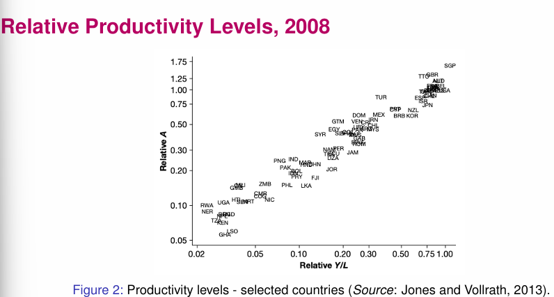
Relative productivity levels and application + analysis:

• Rich countries have high levels of technology

• Strong correlation between relative A and relative Y

  • rich countries have high physical and human capital + productive use of such input

• Correlation is flawed; some countries have level of A much higher than expected

  • suggests we have not controlled other factors adequately enough

  • Our estimates of A should be considered as estimates of Total Factor Productivity

Interpretating Results of relative productivity levels on a global scale:

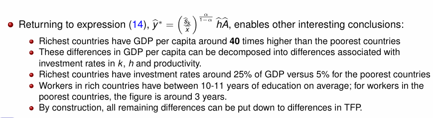
• Rich countries have GDP per capita 40x higher than the poorest countries

  • decomposed into differences of investment rates in k, h and productivity

• Rich countries have investment rates around 25% of GDP vs 5% for the poorest countries

• Workers in rich countries have 10-11 years of education on average vs 3 years for poorest countries

• All remaining differences can be put down to TFP differences

Conclusion of Augmented Solow Model:

Extending the Solow framework to include human capital improves the model’s empirical performance by allowing both physical capital and human capital to drive income differences across countries.

Conditional Convergence with data, + principle of transition dynamics:

• Neoclassical model predicts that among countries with the same steady state, the convergence hypothesis should hold: poor countries SHOULD grow faster

• All countries do not have the same investment, pop growth or tech levels, so they are not expected to grow toward the same steady-state.

• In 1960, good examples of these countries were Japan, Botswana, and Taiwan — economies that grew rapidly over the next forty years, just as the neoclassical model would predict.

• Principle of transition dynamics:

  • The further an economy is below its steady state, the faster the economy should grow.

  • The further an economy is above its steady state, the slower the economy should grow.

Convergence in long-run economic growth: evidence and evaluation:

• Backward countries would tend to grow faster than rich countries, to close the economic gap between the two groups (Gerschenkron 1962 and Abramovitz 1986)

• Are cross-country differences in GDP per capita shrinking overtime?

Evidence of convergence

• Convergence of growth rates between industrialized economies in the long-run:

  • economies that were relatively rich in 1870 (e.g. UK) grew most slowly

  • while countries that were relatively poor (e.g. Japan) grew most rapidly (Figure 4).

• The convergence hypothesis also works well to explain growth rates across the OECD between 1960 and 2008 (Figure 5).

• However, the convergence hypothesis does not explain differences in growth rates across the world as a whole (Figure 6).

Across large samples of countries, it does not appear that poor countries grow faster than rich countries. The poor countries are NOT closing the gap in per capita incomes

Solow Production Framework of Endogenous Growth:

Solow Production Framework

$$Y=K^α(AL)^1−^α$$

• A = level of technology

• α∈(0,1): capital share of income

Tech evolves exogenously:

$$A_t=A_0e^g.^t$$

• At: technology at time t

• A0: initial technology

• g: constant exogenous growth rate of technology

• e: base of natural logarithms

• LR per capita growth = g, policy does not affect LR growth

$$Y=K^α(AL)^1−^α$$

• A = level of technology

• α∈(0,1): capital share of income

Tech evolves exogenously:

$$A_t=A_0e^g.^t$$

• At: technology at time t

• A0: initial technology

• g: constant exogenous growth rate of technology

• e: base of natural logarithms

• LR per capita growth = g, policy does not affect LR growth

The AK Model as part of Exogenous Growth:

Production**: Y = AK,** in which A > 0 (constant productivity parameter)

MPC: dY / dK = A

• dY / dK = derivative of output w.r.t capital —> no diminishing returns

Capital Accumulation and steps to calculate growth rate:

Capital Accumulation

$$K˙=sY−δK$$

• K˙: time derivative of K (change in capital)

• s∈(0,1): saving rate

• δ>0: depreciation rate

Step 1: Substitute Y = AK

K˙=sAK−δK

Step 2: Divide by K

K˙ / K (growth rate of capital) =sA−δ

Step 3: Since Y = AK

Y. / Y = K. / K (cancels out), so the GR = g = sA−δ; saving permanently increases growth

Step 1: With population growth, let L. / L = n

• n = population growth rate

Step 2: Define capital per worker

k = K / L

capital per worker evolves as k˙=sAk−(δ+n)k

Step 3: rearrange to get k./k

Growth rate: k˙/k = sAk−(δ+n)

Arrow’s Learning-by-Doing Model of Exogenous Growth and steps to find Y:

Production:

$$Y=BK^αL^1−^α$$

• B: knowledge externality term

• α: capital share

Step 1: Knowledge accumulation

$$B=AK^1−^α$$

Step 2: Substitute into Y

$$Y=AKL^1−^α$$

if L = 1, then Y = AK, aggregate increasing returns

Increasing returns from fixed costs of Exogenous Growth:

y = 100 (x-F)

• x: labour hours, F: fixed cost, 100: marginal productivity parameter

MP: dy / dx = 100

$$AP: y / x = 100(x-F) / x$$

As x increases —> AC falls —> increasing returns

Romer Model of Exogenous Growth: FG production, Capital Accumulation and Pop Growth:

Final Goods Production

$$Y=K^α(AL_Y)^1−^α$$

• LY: labour in goods production, A: idea stock

Capital Accumulation

$$K˙=sY−dK$$

• d: depreciation rate

Population Growth

L˙ / L = n

Production of Ideas: Basic idea creation, Knowledge spillover parameters, duplication effects and Labour allocations

Basic Idea Creation

$$A˙=δL_A$$

A˙: new ideas per period, LA = researchers and δ >0 ; research productivity parameter

Knowledge Spill-overs

$$A˙=δA^ϕL_A$$

ϕ: knowledge spill-over parameter

• ϕ>0: research becomes easier

• ϕ<0: fishing-out effect

Duplication Effect

$$A˙=δA^ϕL^λ_A$$

0<λ<1: duplication parameter

• smaller λ → more overlap between researchers

Labour Allocation

$$L = L_A + L_Y$$

• Total labour split between research and production

• Research share: LA / L = SR

  • S_R: share of labour in R&D

  • LA = S_RL

Balanced Growth Rate (BGP) of Exogenous Growth:

On BGP:

$$gY = gK = gA$$

• gY: growth rate of output

• gK: growth rate of capital

• gA: growth rate of technology

To derive gA:

• divide by A, take logs, differentiate w.r.t time, on BGP LA˙ / LA = n, then substitute and solve to get gA =λn / 1−ϕλn

Growth Formula for Exogenous Growth, including parameters from pop, dup and knowledge:

$$gA=λn / 1−ϕ$$

Growth depends on:

• n: population growth

• λ: duplication effect

• ϕ: knowledge spillovers

Research share SR does NOT affect LR growth

Special case of Growth Formula

If λ=1 and ϕ=0

Then: gA=n

Steady State Growth Per Capita For Exogenous Growth:

• Long-run per capita growth = population

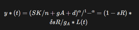
y∗(t)=(SK /n+gA+d)^α/^1-^α =(1−sR)δsR/g_AL(t)

• y(t):* steady-state output per worker at time t

• sK: saving rate

• d: depreciation

• gA: technology growth

• sR: research share

• L(t): population level

Effects of Increasing Research Share For Exogenous Growth:

Increase sR:

Short run:

$$gA=δLA/A$$

jumps upward.

Long run:

gA→λn / 1−ϕ

• Growth unchanged and higher permanent level of A

  • This is a level effect, not a growth effect

Core Theoretical Conclusions from the Exogenous Growth Theory:

1. Growth arises from purposeful R&D.

2. Ideas are non-rival → increasing returns.

3. Long-run growth determined by: g=λn / 1−ϕ

4. Research intensity affects levels.

5. Population scale sustains growth.

6. Knowledge spillovers are fundamental.