Econ Exam 2

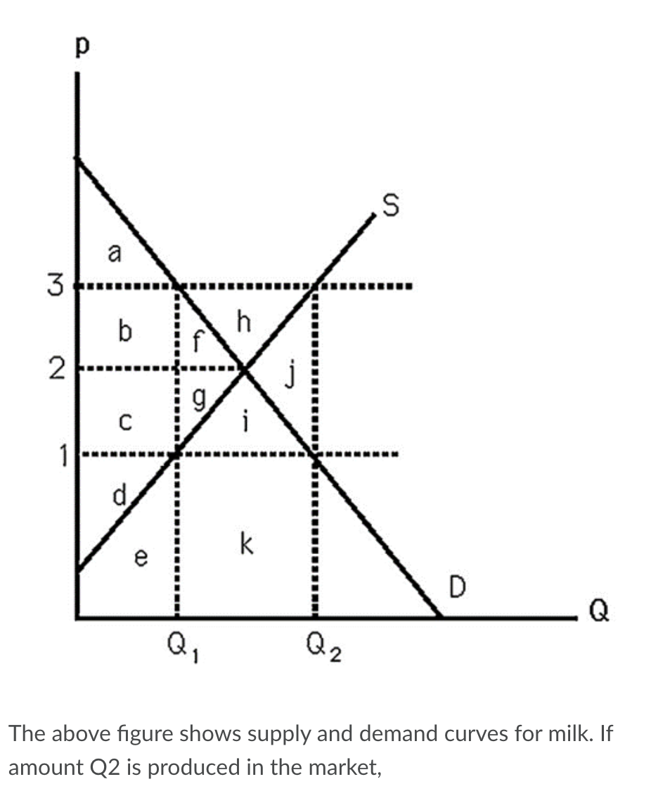
In the very short run,

quantity supplied is absolutely fixed.

In the short run,

existing firms may change the quantity they are supplying.

Scenario 10-1

​

Suppose domestic beef producers face demand of Q_D = 100 – 5P.

Refer to Scenario 10-1. In the very short run, 50 pounds of beef are produced. Suppose mad cow strikes a portion of the national herd and the amount brought to market falls to 40. The price per head will rise by

$2

The short-run market supply curve is

the horizontal summation of each firm's short-run supply curve.

Scenario 10-3

​

Suppose there are 100 firms each with a short-run total cost of STC = q² + q + 10, and the short-run supply curve for each firm is q = 0.5P - 0.5.

Refer to Scenario 10-3. The market supply curve is

Q_S = −50 + 50P

Scenario 10-3

​

Suppose there are 100 firms each with a short-run total cost of STC = q² + q + 10, and the short-run supply curve for each firm is q = 0.5P - 0.5.

Refer to Scenario 10-3. If market demand is given by Q_D = 1,050 − 50P, what is the equilibrium price?

$11

Scenario 10-3

​

Suppose there are 100 firms each with a short-run total cost of STC = q² + q + 10, and the short-run supply curve for each firm is q = 0.5P - 0.5.

Refer to Scenario 10-3. If market demand is given by Q_D = 1,050 − 50P, how much will be produced in the market?

500

Scenario 10-3

​

Suppose there are 100 firms each with a short-run total cost of STC = q² + q + 10, and the short-run supply curve for each firm is q = 0.5P - 0.5.

Refer to Scenario 10-3. If market demand is given by Q_D = 1,050 − 50P, how much will the individual firm produce?

5

In the short run, an increase in market demand will usually lead to

an increase in price and an increase in quantity.

A demand curve will shift out for any of the following reasons except:

Price of a substitute falls.

If a 1 percent increase in price leads to a 0.7 percent increase in quantity supplied in the short run, the short-run supply curve is

inelastic.

If the market for hula-hoops is characterized by a very inelastic supply curve and a very elastic demand curve, an inward shift in the supply curve would be reflected primarily in the form of

lower output.

If the market for bottled spring water is characterized by a very elastic supply curve and a very inelastic demand curve, an outward shift in the supply curve would be reflected primarily in the form of

lower prices.

Under perfect competition, if an industry is characterized by positive economic profits in the short run,

firms will enter the market in the long run and the short-run supply curve will shift outward.

Positive economic profits exist for a firm in the long run if price is above

long-run average cost.

Firms in long-run equilibrium in a perfectly competitive industry will produce at the low points of their average cost curves because

firms maximize profits and free entry implies that maximum profits will be zero.

Scenario 10-4

 

Suppose demand for a good is Q_D = 100 – P and supply is Q_S = –20 + P.

Refer to Scenario 10-4. What is the equilibrium price?

$60

Scenario 10-4

 

Suppose demand for a good is Q_D = 100 – P and supply is Q_S = –20 + P.

 Refer to Scenario 10-4. What is the equilibrium quantity?

40

a positive

Long-run elasticity of supply is defined as

percentage change in quantity supplied in the long run divided by percentage change in price.

In a competitive market, an efficient allocation of resources is characterized by

the largest possible sum of consumer and producer surplus.

Scenario 10-4

 

Suppose demand for a good is Q_D = 100 – P and supply is Q_S = –20 + P.

Refer to Scenario 10-4. What is the amount consumers pay producers?

$2,400

Scenario 10-4

 

Suppose demand for a good is Q_D = 100 – P and supply is Q_S = –20 + P.

Refer to Scenario 10-4. What is the consumer surplus?

$800

In the short run, the incidence of a sales tax is

shared between the consumer and the producer.

In an increasing cost industry, the greater burden of a specific tax will usually be absorbed in the long run by

the party with the least elastic demand/supply curve.

In the short run, specific taxes on a firm result in

an increase in the price paid by consumers.

The excess burden of a tax is

the loss of consumer and producer surplus that is not transferred elsewhere.

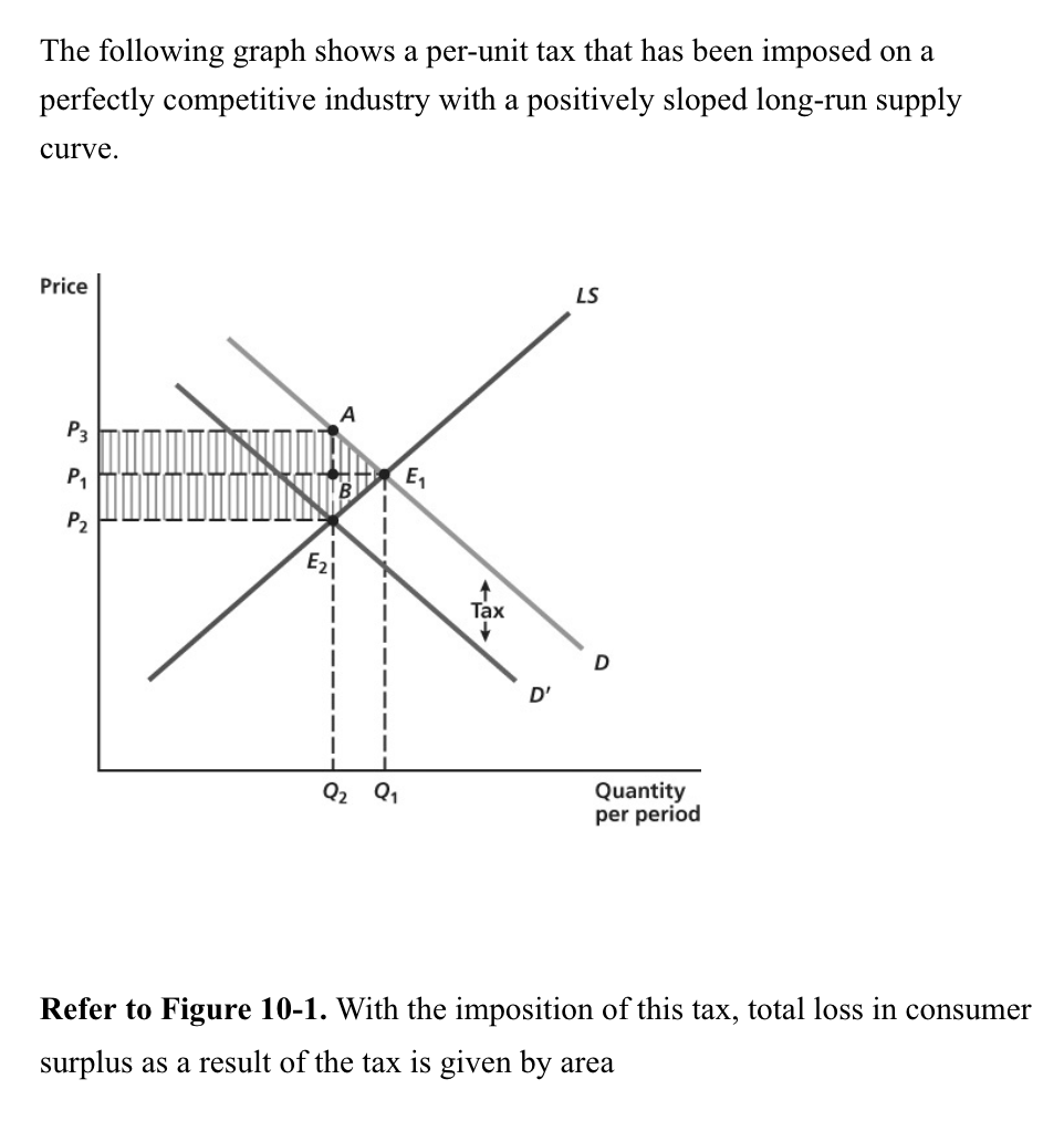
P₃AE₁P₁.

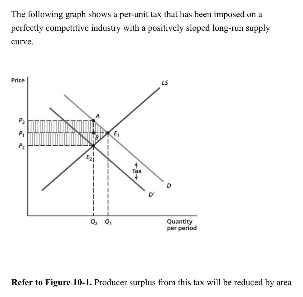
P₁E₁E₂P₂.

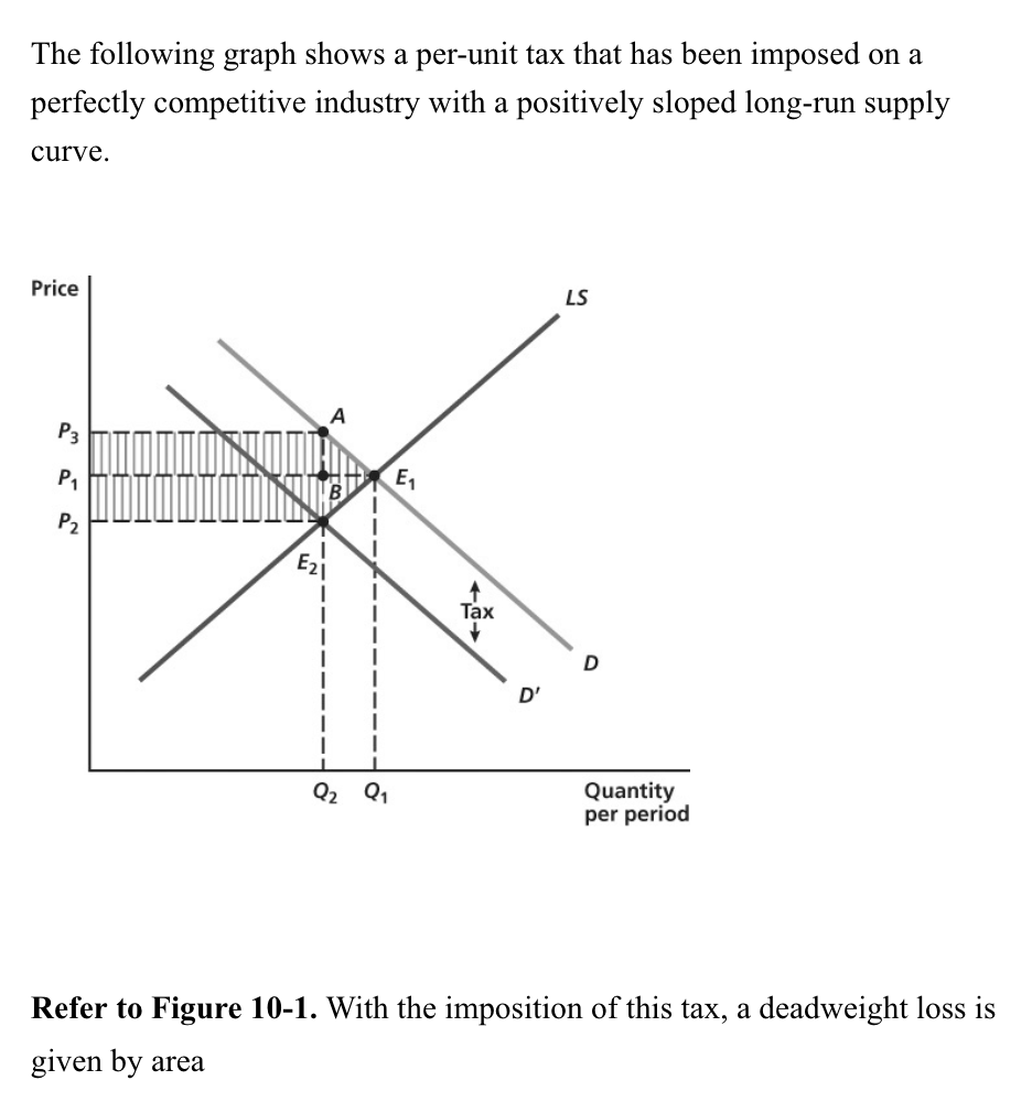
AE₁E₂.

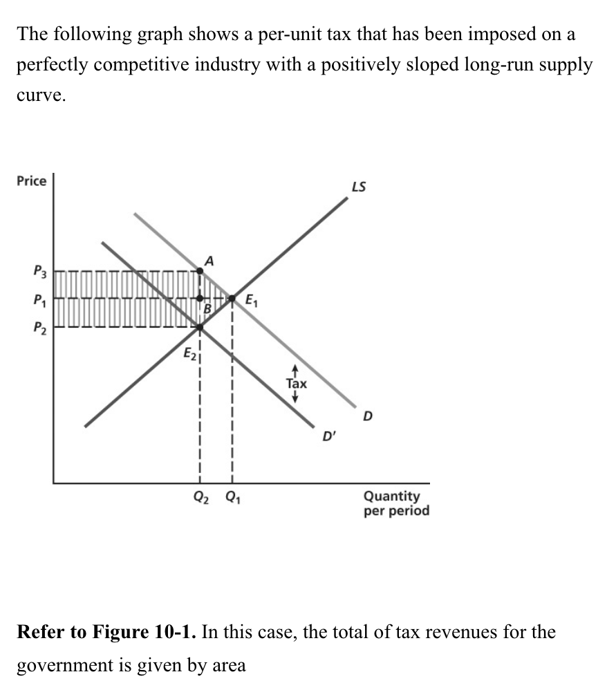
P₃AE₂P₂.

a deadweight loss is generated.

Suppose the market supply curve is p = 5 + Q. At a price of 10, producer surplus equals

12.50

The slope of the production possibility frontier shows

the opportunity cost of production of more of one good in terms of the other good.

The slope of the production possibility frontier also shows

how production of one good can be substituted for another while still using a fixed supply of inputs efficiently.

At a perfectly competitive equilibrium with production and trade, the slope of the production possibility frontier will be

equal to the slope of the isovalue line

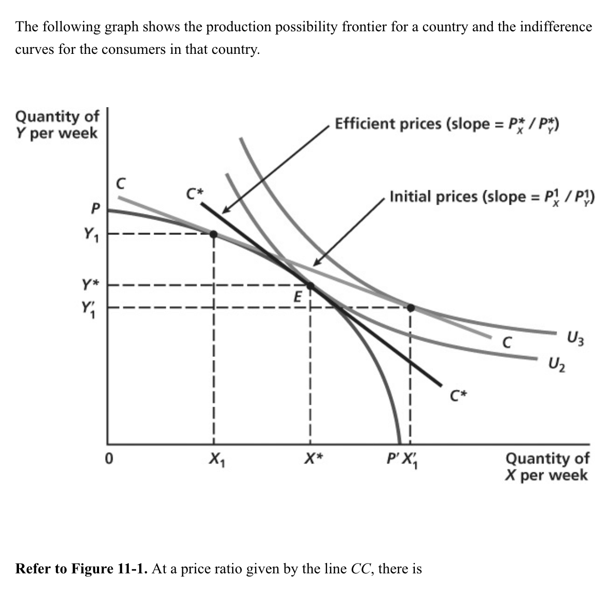
an excess demand for good X and an excess supply for good Y.

Each of the following factors might interfere with the efficiency of perfect competition except:

diminishing marginal product.

The reason externalities distort the allocation of resources is that

a firm’s private costs do not reflect the social cost of production.

Markets can fail to achieve efficiency when

there are public goods.

Markets can fail to achieve efficiency when

there are markets with imperfect competition.

Markets can fail to achieve efficiency when

there are buyers or sellers without adequate information about the quality of goods.

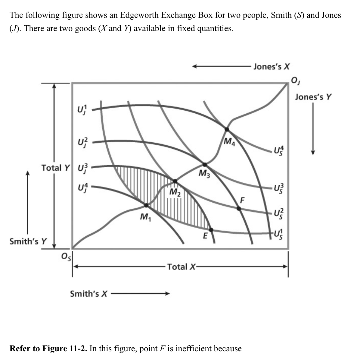
both persons could be made better off by moving to a point between M₂ and M₃.

raise both persons' utility.

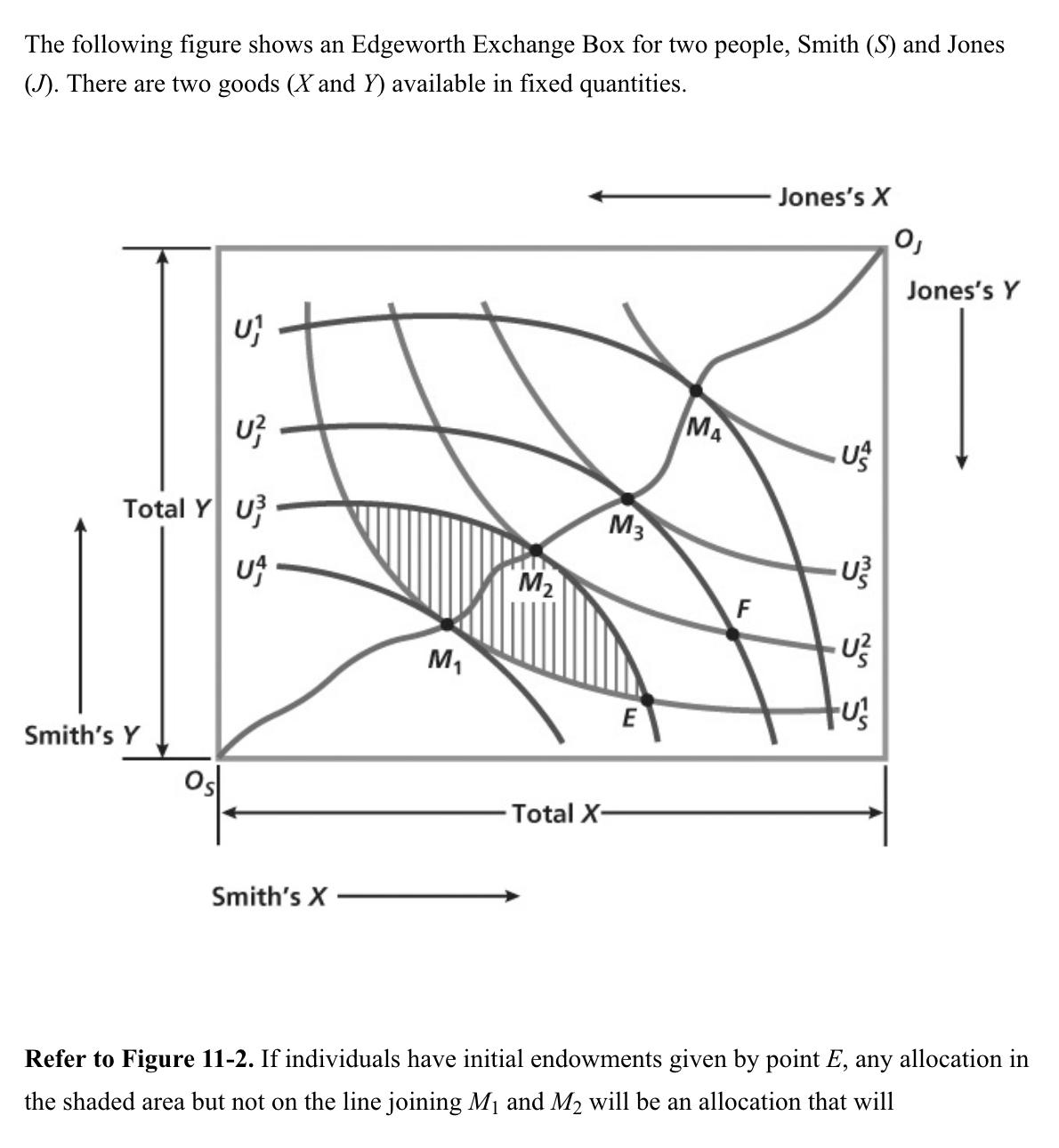
be inefficient because both people can still be made better off.

Moving away from the contract curve will

harm at least one of the parties.

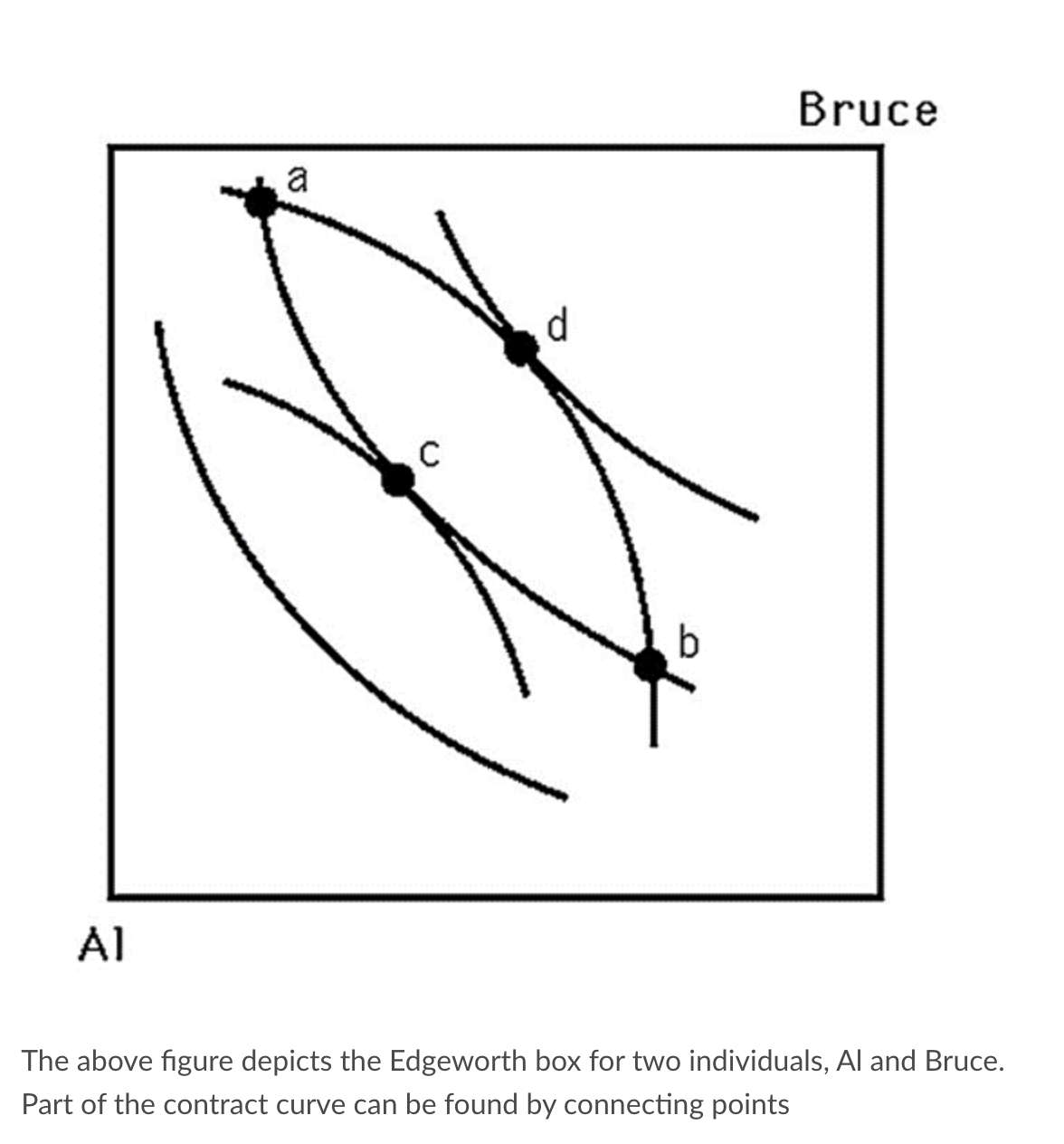
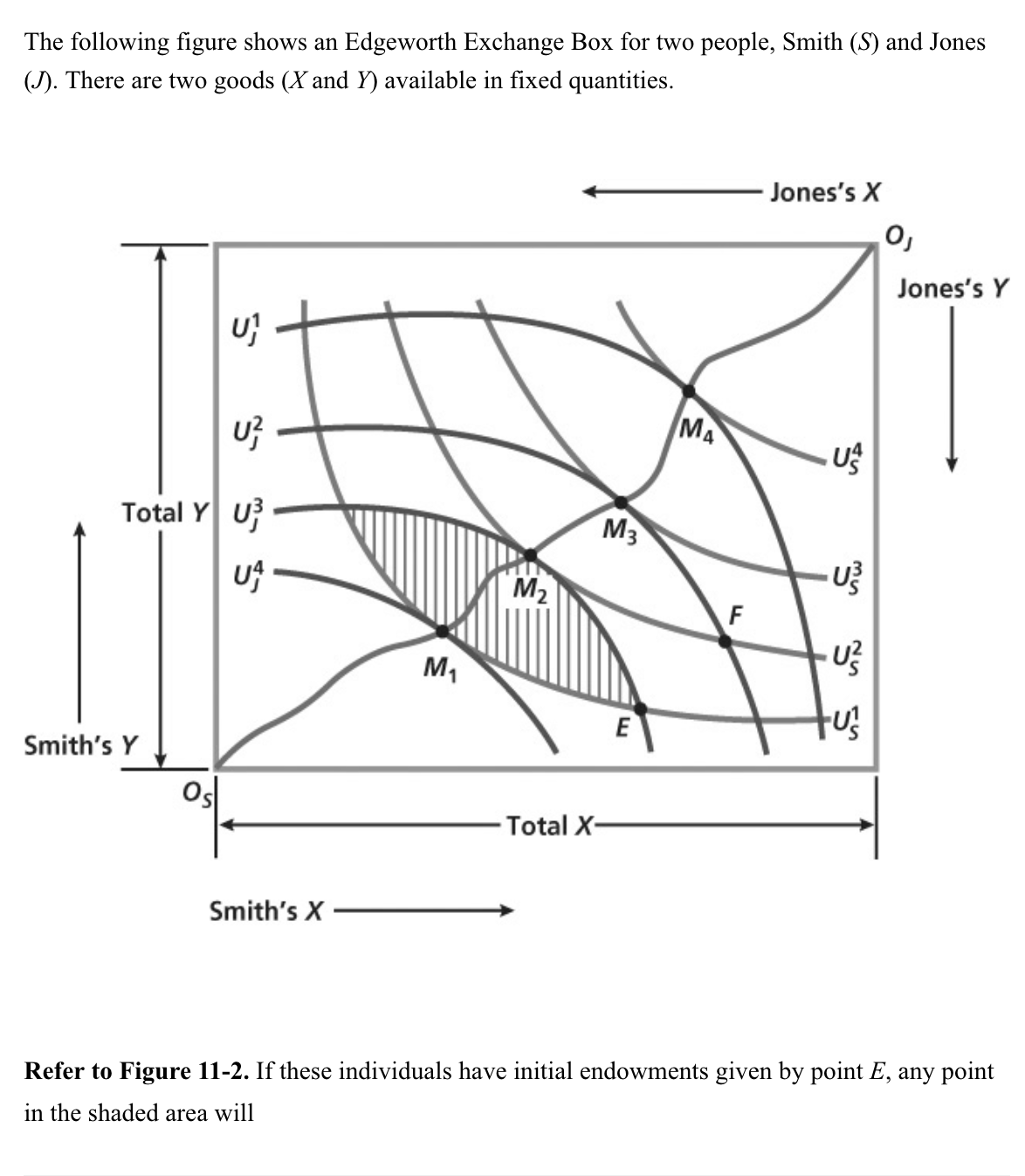
c and d.

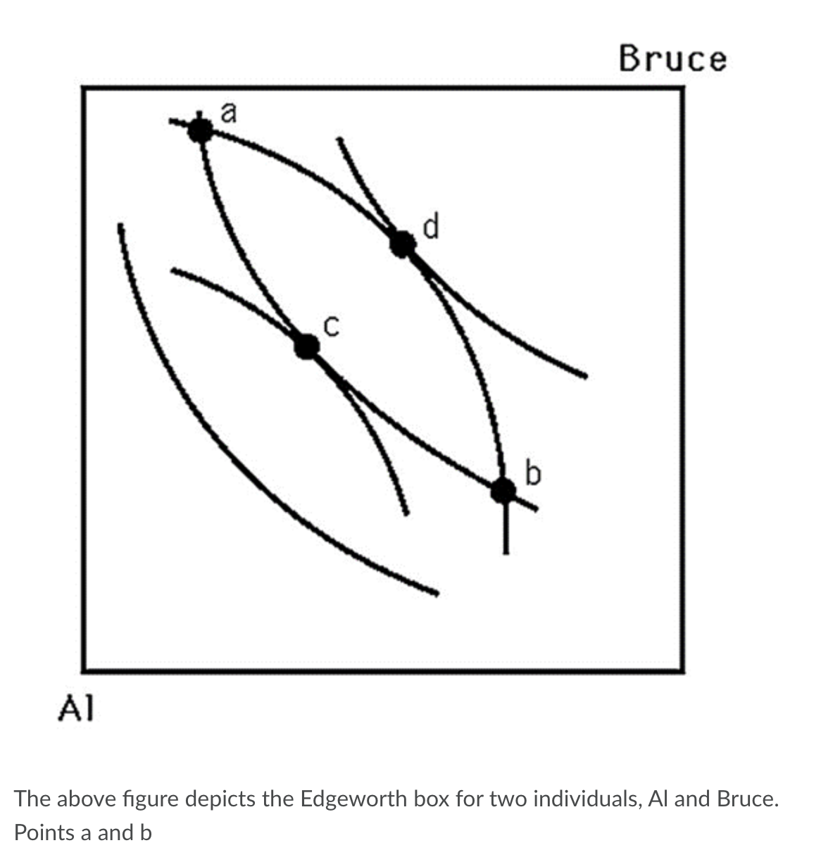
are definitely not the final allocations after trading.

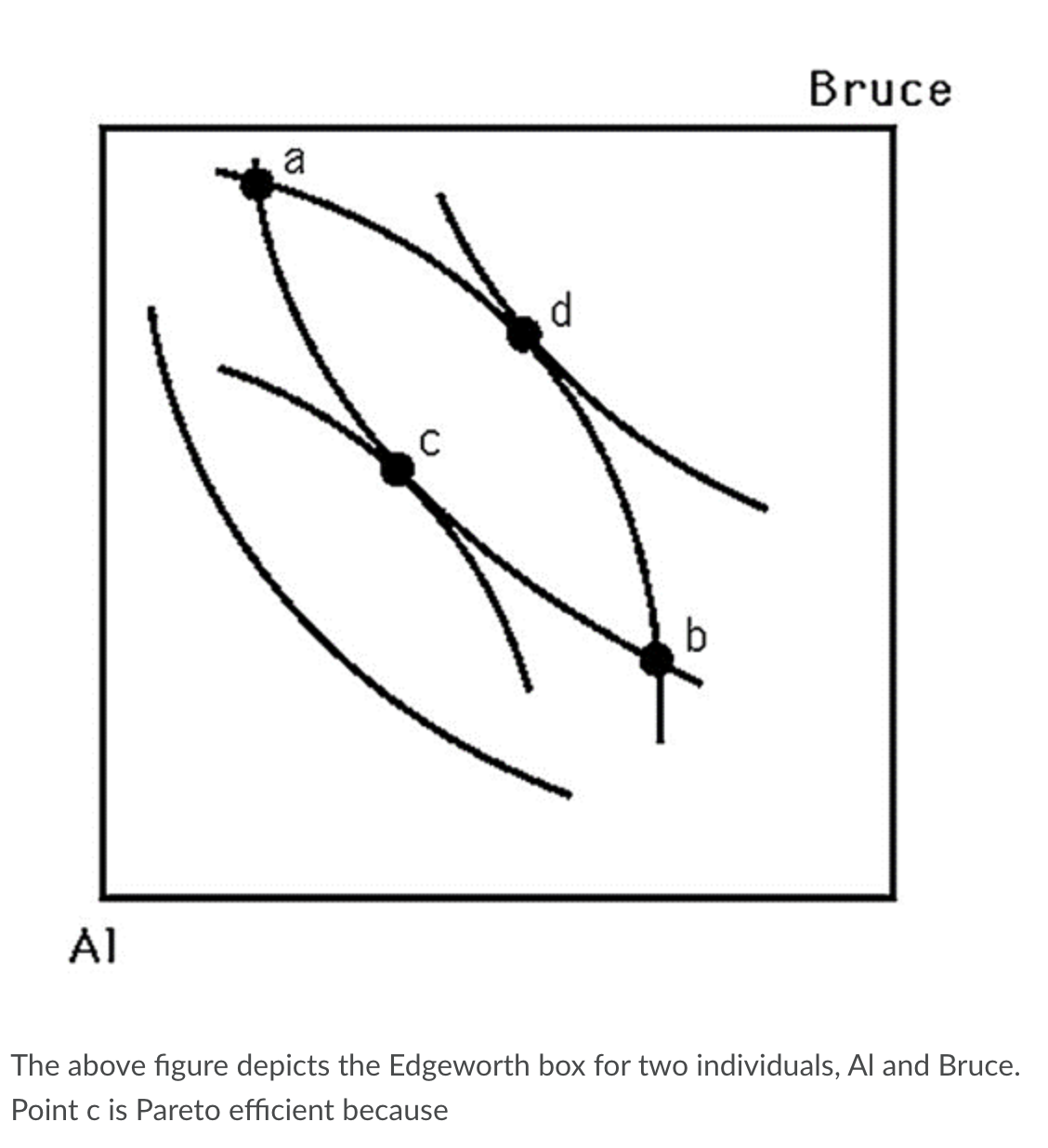
the MRS's are equal.

the indifference curves are tangent. 

no mutual gains from trade exist.

The fact that any Pareto-efficient equilibrium can be achieved through competition by adjusting initial endowments is called

the Second Welfare Theorem.

A game in economics is defined as

competition in which strategic decision making is integral.

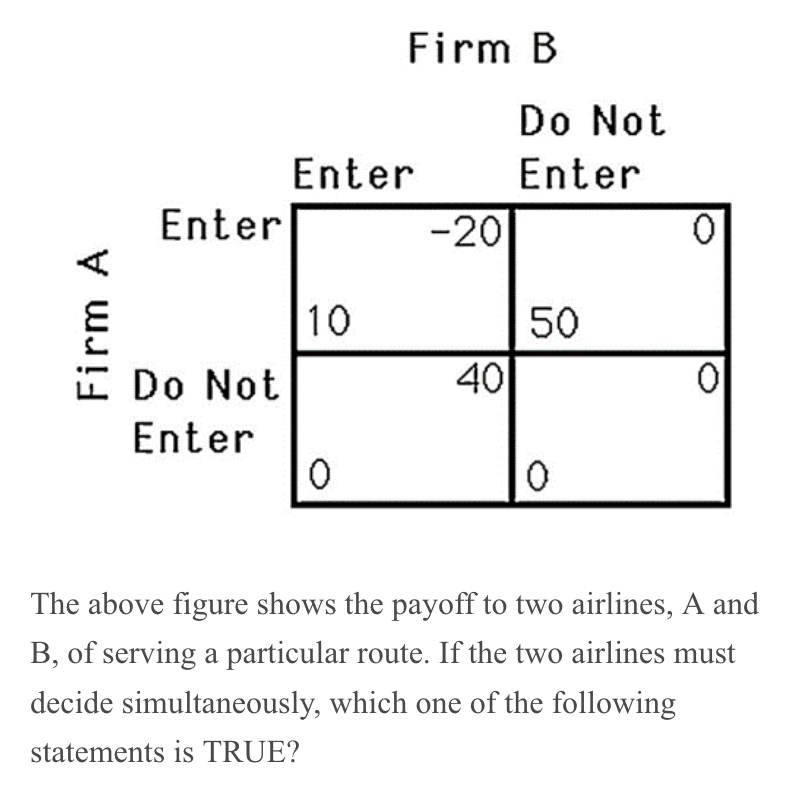
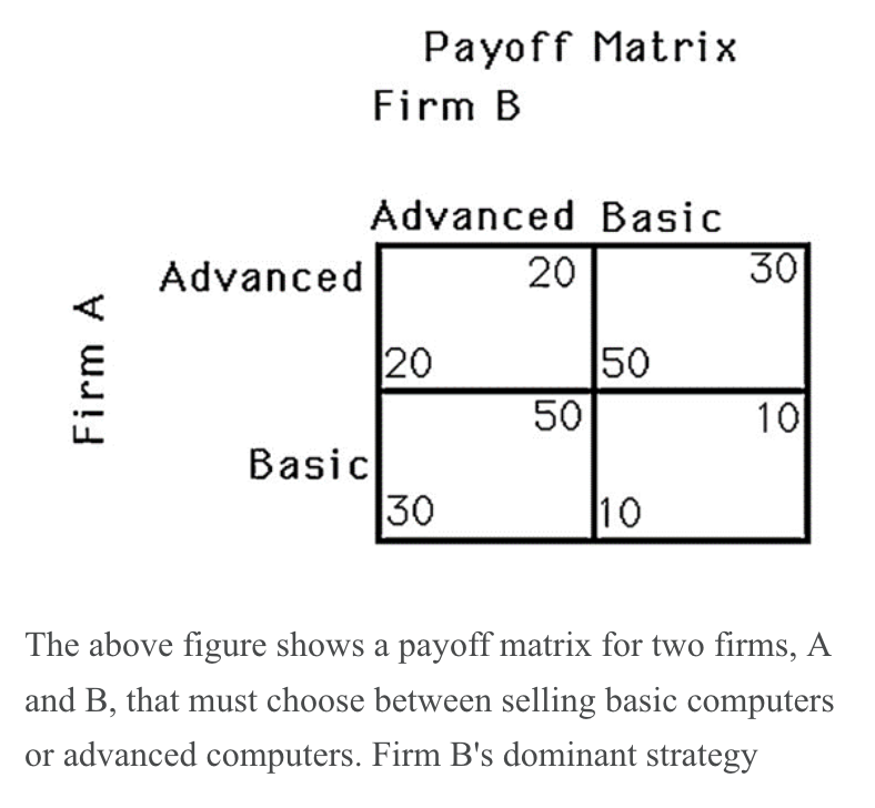
Firm B does not have a dominant strategy.

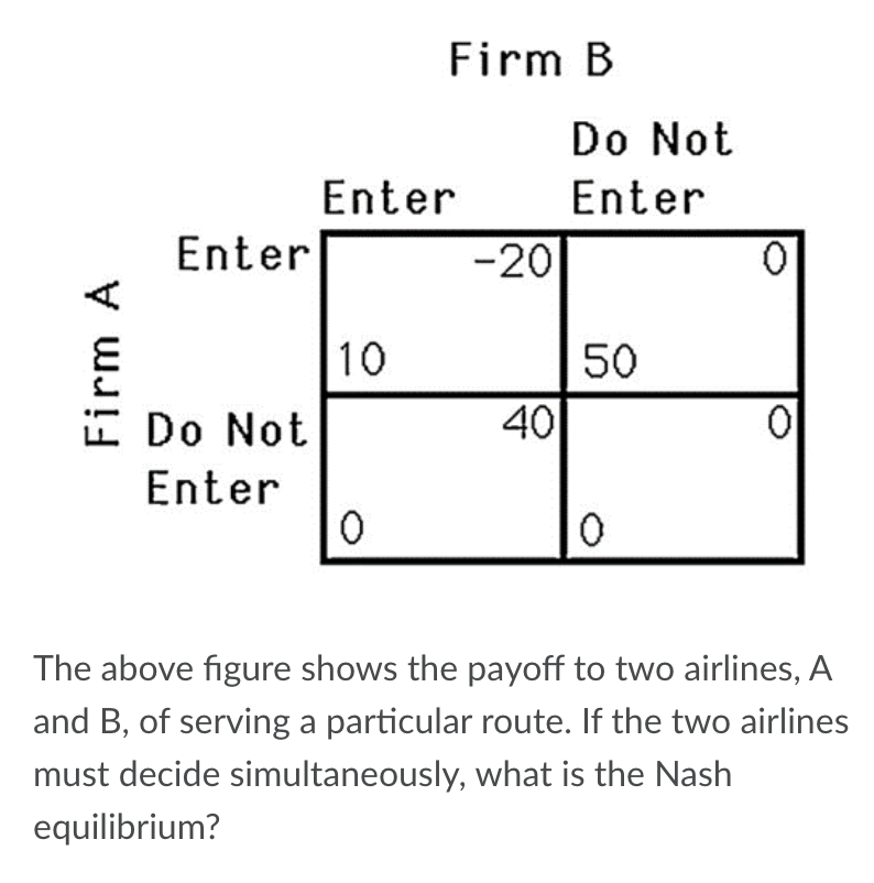
Firm A enters but Firm B does not enter

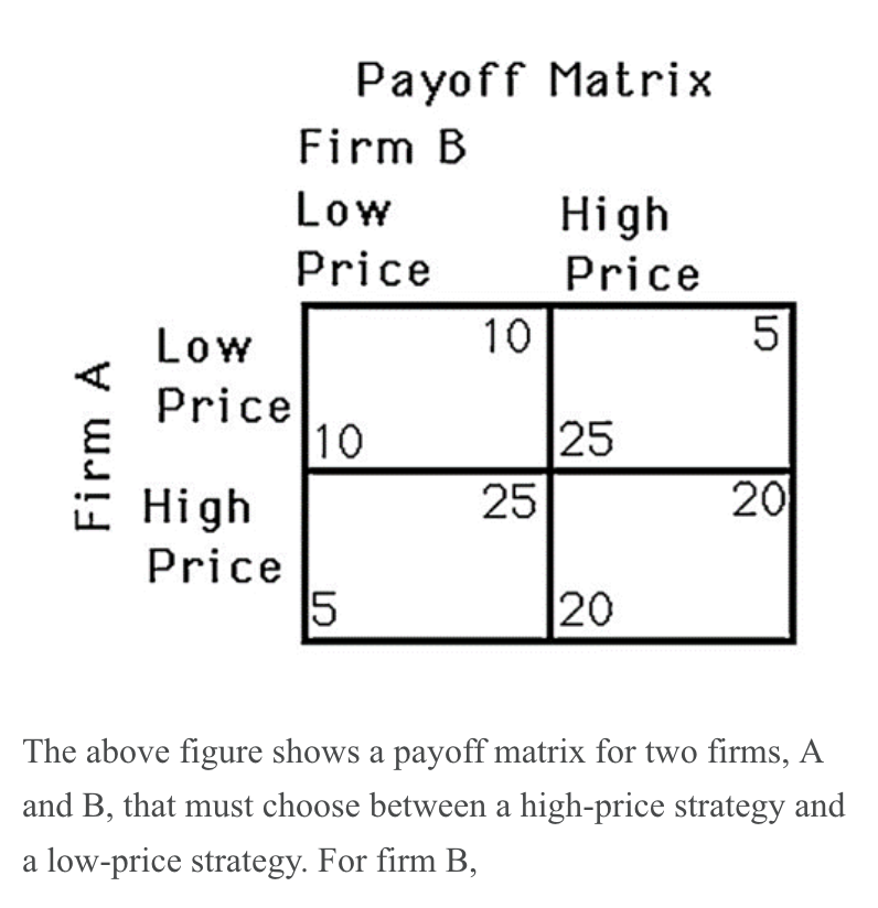
setting a low price is the dominant strategy.

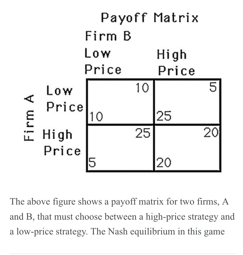
occurs when both firms set a low price.

does not exist in this game.

In a non-cooperative, imperfect information, simultaneous-choice, one-period game, a Nash equilibrium

may not maximize the sum of the firms' profits.

Suppose there are two firms, Boors and Cudweiser, each selling identical-tasting nonalcoholic beer. Consumers of this beer have no brand loyalty so market demand can be expressed as P = 5 – 0.001(Q_B + Q_C). Boors’ marginal revenue function can be written MR = 5 – 0.001(2Q_B + Q_C) and symmetrically for Cudweiser. Both firms have constant costs of $2 per unit (MC = AC = 2.)

Refer to Scenario 13-1. Assuming the firms behave as Cournot competitors, in the Nash equilibrium, Cudweiser will produce

1,000

Suppose there are two firms, Boors and Cudweiser, each selling identical-tasting nonalcoholic beer. Consumers of this beer have no brand loyalty so market demand can be expressed as P = 5 – 0.001(Q_B + Q_C). Boors’ marginal revenue function can be written MR = 5 – 0.001(2Q_B + Q_C) and symmetrically for Cudweiser. Both firms have constant costs of $2 per unit (MC = AC = 2.)

Refer to Scenario 13-1.Assuming the firms behave as Cournot competitors, in the Nash equilibrium, Boors will produce

1,000

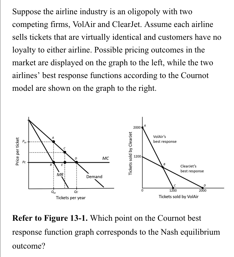
B

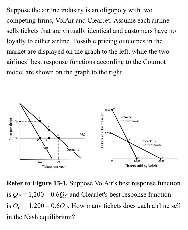
VolAir sells 750, and ClearJet sells 750.

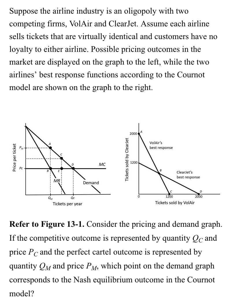
C

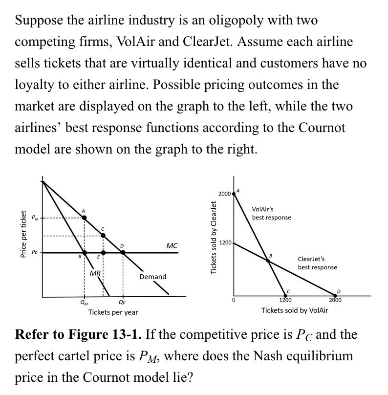
Between P_M and P_C

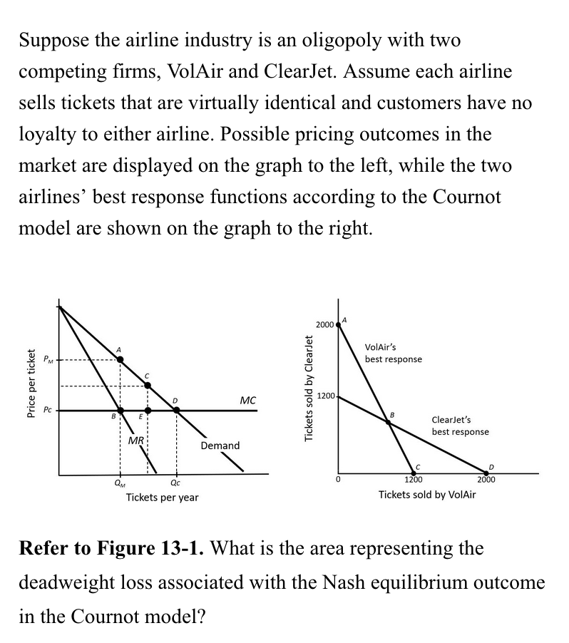
CED

In the cartel model,

firms coordinate their decisions to act as a monopoly.

Under the cartel model, each firm produces where

marginal cost equals marginal revenue.

The Cournot Model of Oligopoly assumes that

All of the above.

Compared to a cartel, firms in a Cournot Oligopoly

make less joint profit.

Assuming a homogeneous product, the Bertrand duopoly equilibrium price is

less than the Cournot equilibrium price.

In a Bertrand model with identical firms and a non-differentiated product, price will increase in response to

an increase in marginal cost.

An input’s marginal revenue product is given by

the input’s marginal product times marginal revenue of the firm’s output.

The notion that when the price of an input falls, a firm’s marginal cost curve shifts down and overall production increases so that more of every input is employed is known as

the output effect.

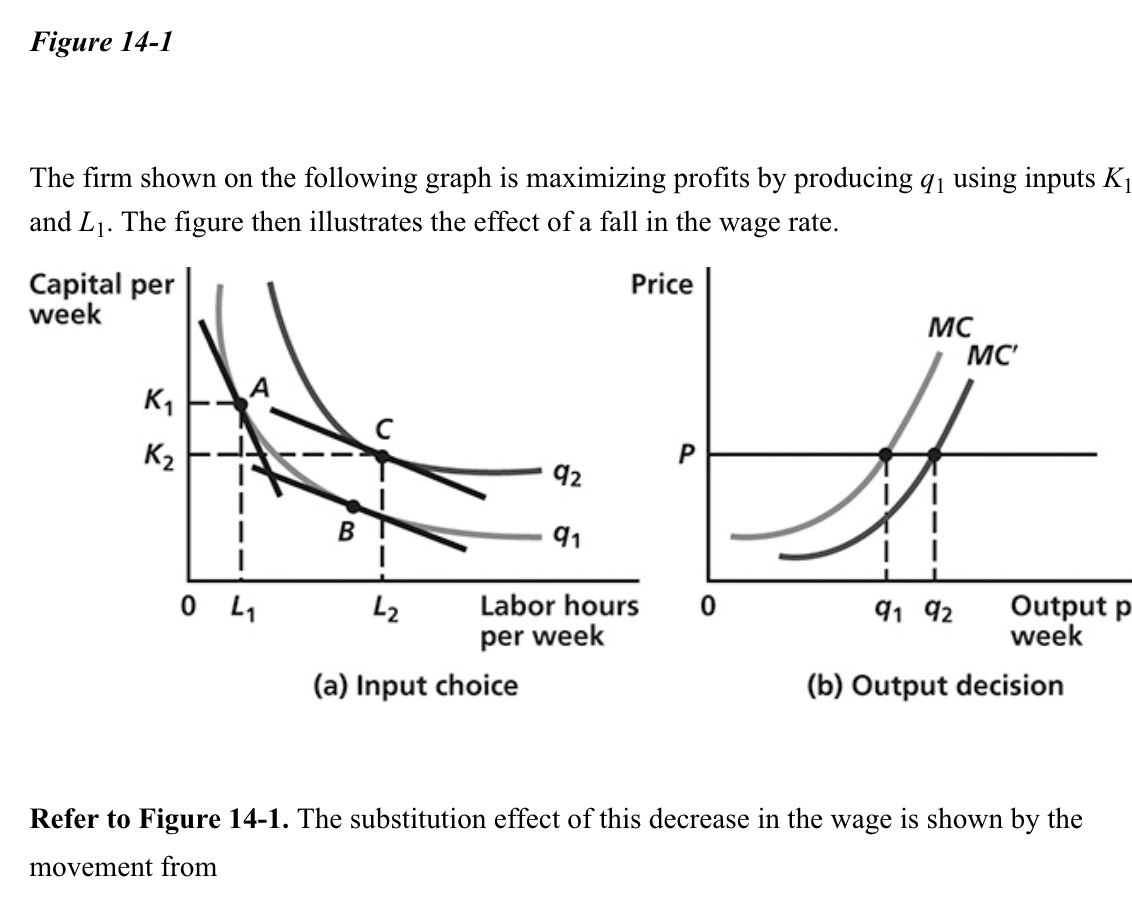
A to B

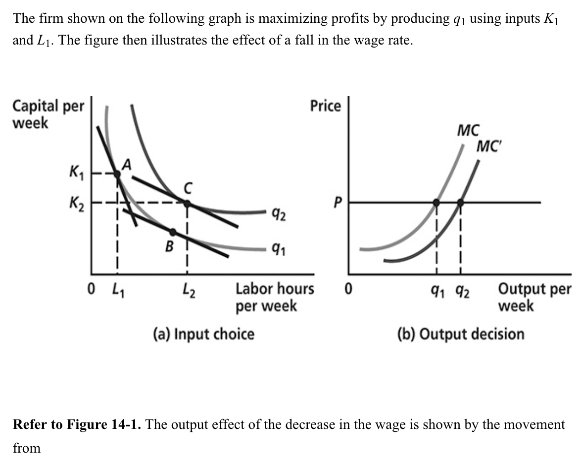
B to C

If the price of an input falls, what are the two reasons a firm would increase the use of that input?

Overall production costs are now lower and the firm can substitute this input for other relatively more expensive inputs.

The output effect of a change in the wage rate on a firm’s demand for labor input will be greater

the larger the share of labor costs in total costs and the greater the price elasticity of demand for output.

The size of the reduction in quantity of labor hired by a firm due to an increase in the wage rate depends upon all of the following except

the capital to labor ratio before the wage increase.

Suppose the market for labor is perfectly competitive and the demand for labor is L = 100 – 10w and market supply is L = –20 + 10w.

Refer to Scenario 14-2. The equilibrium wage will be

6 dollars

Suppose the market for labor is perfectly competitive and the demand for labor is L = 100 – 10w and market supply is L = –20 + 10w.

Refer to Scenario 14-2. The equilibrium number of workers hired will be

40

Suppose the market for labor is perfectly competitive and the demand for labor is L = 100 – 10w and market supply is L = –20 + 10w.

Refer to Scenario 14-2. If a minimum wage is imposed at w = 8, the number of workers hired will be

20

Suppose the market for labor is perfectly competitive and the demand for labor is L = 100 – 10w and market supply is L = –20 + 10w.

Refer to Scenario 14-2. If a minimum wage is imposed at w = 8, the total unemployed (L_S – L_D) will be

40

A firm will hire additional units of any input up to the point where

the expense of employing the last unit is equal to the revenue brought in by the last unit.

If a firm is a monopsonistic hirer of labor,

its marginal expense for labor is greater than the market wage.

A monopsonist who is a price taker in an output market will hire labor up to the point where

the marginal expense of labor is equal to the marginal value product of labor.

For a monopsonistic hirer of labor, the gap between labor’s marginal value product and its wage rate will be greater

the more inelastic the supply curve for labor.