Statistical Inference

What are descriptive statistics and inferential statistics?

Descriptive statistics are basic summaries of observed data. Typically, it is not assumed that the observed data have originated from any probability distribution

e.g. mean, s.d., median, bar charts, histograms

Inferential statistics aims to make inference about a population from the sampled data. Typically involves assuming a probability distribution for some outcome of interest (but not always!)

e.g. confidence intervals, hypothesis testing, linear models, ANOVA

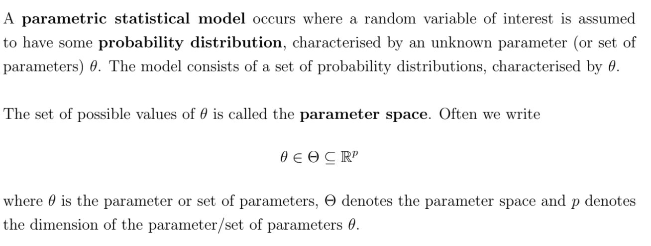
What is a parametric model and the parameter space?

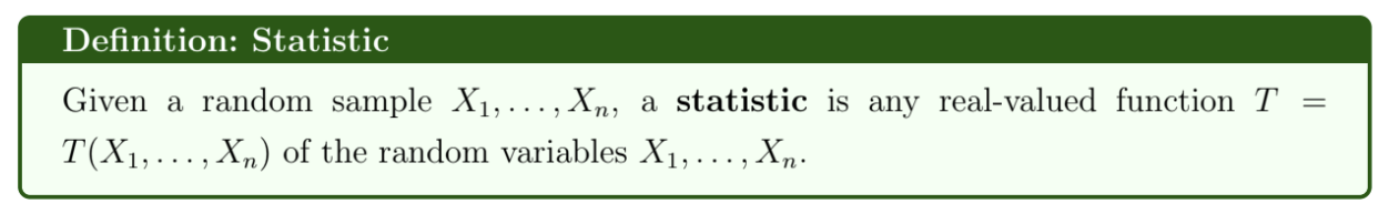
What is a statistic?

e.g. sample mean, sample variance, sample maximum

T(X) is a function of random variables and so is a random variable itself

The probability distribution of T(X) is its sampling distribution.

What is the estimator, estimand and estimate?

An estimator of the parameter $\theta$ is a statistic T(X) used to estimate $\theta$. The estimator is a random variable

The estimand is the parameter $\theta$ we are trying to estimate

The estimate is the realised value of T(X), i.e. the statistic of the data actually observed

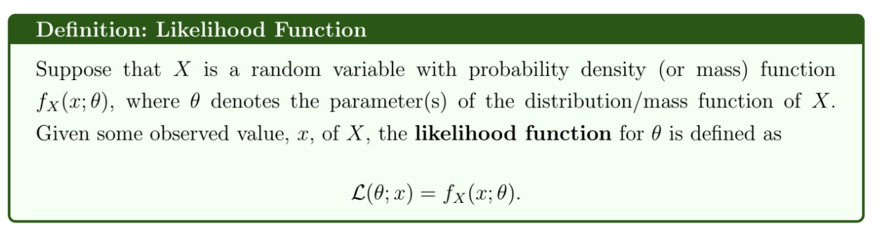
What is the likelihood function?

The likelihood function is the probability density / mass function of X, but considered to be a function of $\theta$ for fixed X

For multiple observations X, the likelihood is the joint probability density / mass function of X. If the values of Xi are independent, it is the product of their pdf/pmfs.

What is the invariance property of a maximum likelihood estimate?

If $\hat{\theta}$ is a maximum likelihood estimate of $\theta$ and g is any function then $g(\theta)$ is a maximum likelihood estimate of $g(\theta)$

Tips for maximum likelihood estimation

Often easier to find $\theta$ that maximises the log-likelihood function

Because the natural logarithm is a strictly increasing function, $\theta$ will also maximise the likelihood function

Take second derivatives of the likelihood to check that the likelihood has been maximised

Note that maximising a likelihood by solving a score equation only finds a local maximum - a global maximum may lie at the boundary of the parameter space

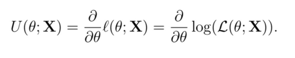
What is the score function?

The score function is the gradient of the log-likelihood function / the first derivative with respect to $\theta$

The score equation sets the score function to zero - solve this to derive maximum likelihood estimates

What is the likelihood principle?

Given a sample of data and an assumed statistical model, then the likelihood principle states that all information from the sample that is relevant to the model parameters is contained within the likelihood function

Moreover, two likelihood functions are equivalent if one is a scalar multiple of the other.

What is a sufficient statistic?

T(X) is sufficient for $\theta$ if the condition probability distribution of $X_{1},…,X_{n}$ given that T(X) = t does not depend on $\theta$

i.e $f\left(x_1,\ldots,x_{n}\vert T\left(x\right)=t\right)$ does not depend on $\theta$

If T(X) is sufficient for $\theta$, then knowing more about the sample than T(X) = t is not necessary for making inference about $\theta$

A maximum likelihood estimator (where it exists) is always a function of a sufficient statistic

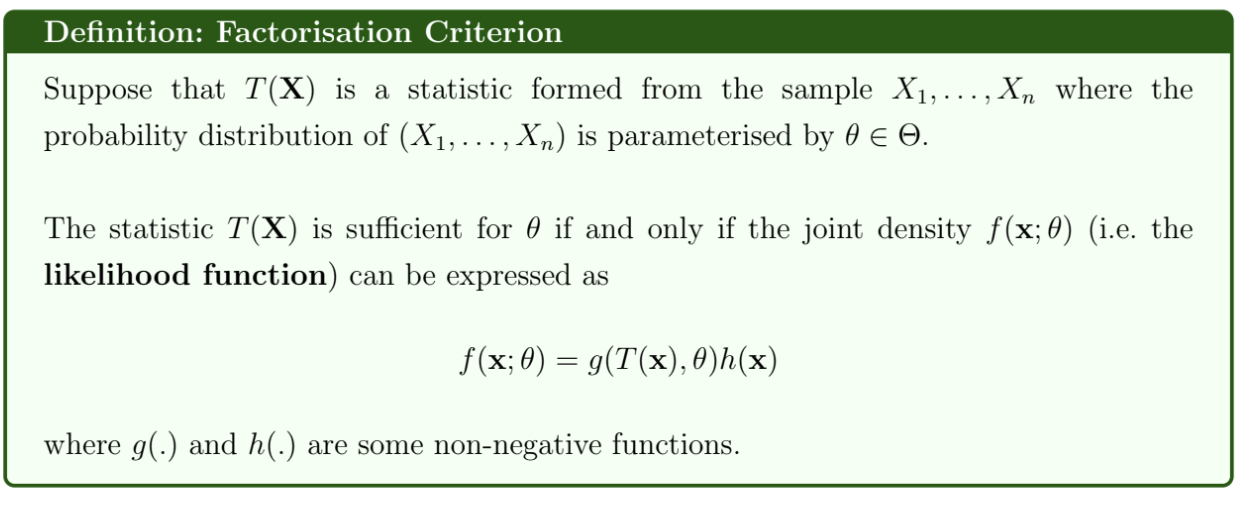
What is the factorisation criterion?

The joint density can be written as the product of g and h, where g depends on $\theta$ and the sufficient statistic, but h does not depend on $\theta$

What is the sufficiency principle?

The sufficiency principle states that if two sets of data x and y result in the same value of a sufficient statistic T (i.e. T(x) = T(y), where T is sufficient for $\theta$) then these sets of data must lead to the same inference on $\theta$

If T is sufficient for $\theta$ then,

1. Any invertible function of T is also sufficient for $\theta$

2. (T, U), where U(X) is any statistic constructed using X, is also sufficient for $\theta$

Therefore, sufficient statistics are not unique

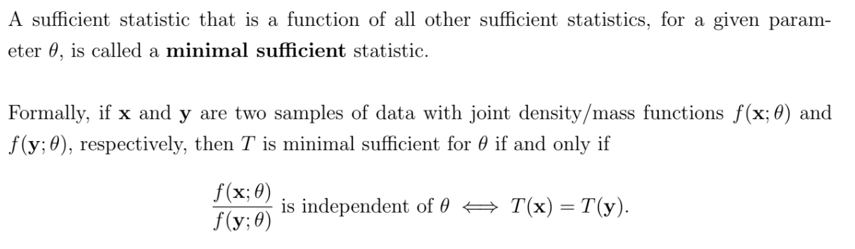
What are minimal sufficient statistics?

A complete and sufficient statistic will also be minimum sufficient

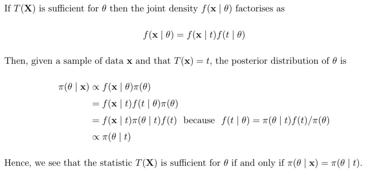
When is a statistic sufficient in a Bayesian context?

How do Frequentist, Likelihood and Bayesian approaches to inference differ?

The frequentist approach regards the true parameter value $\theta$ as fixed but unknown. This approach involves concepts such as unbiased estimators in point estimation and significance levels in hypothesis testing. The properties of the chosen “decision function”, e.g. the point estimator or critical region, depends on the full sample space of x. e.g. if a sample mean $\bar{X}$ is unbiased for $\mu$, this means that the expected value of $\bar{X}$, taken over the whole sample space, is equal to $\mu$

The likelihood approach focuses on the probability of the data actually observed and does not take the rest of the sample space into account. We focus on $f(x;\theta)$ as a function of $\theta$ over the whole parameter space, but only at the single observed data point x.

The Bayesian approach also focuses on the observed data and ignores unobserved points in the sample space. However, the parameter $\theta$ is regarded as random rather than fixed and so is assigned a probability distribution that is intended to reflect beliefs about the value of the parameter.

What is the risk function and Bayes risk?

The risk function is the expected value of a loss function

$$R(\theta, \delta) = E[L(\theta, \delta(X))]$$

The Bayes risk is the expected value of the risk, obtained by integrating the risk function over values of $\theta$. It can be interpreted as the posterior expected loss on taking decision $\delta(x)$, given the observation x.

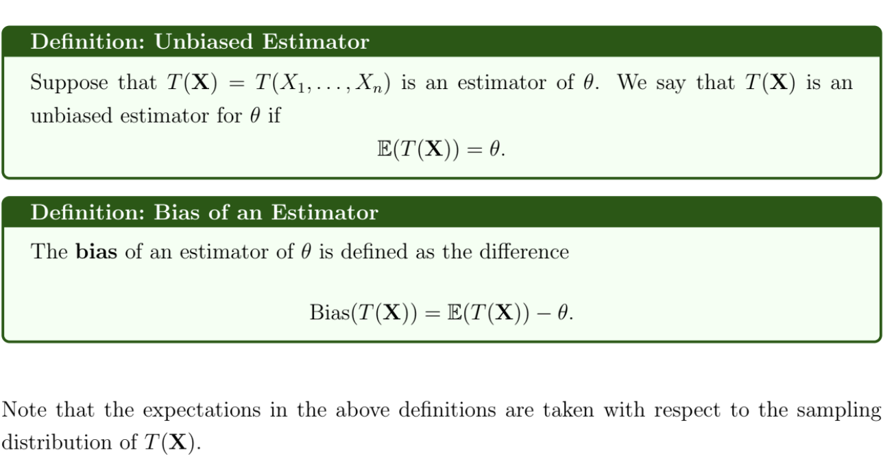
What is an unbiased estimator and what is the bias of an estimator?

Unbiasedness is not invariant - if T is an unbiased estimator for $\theta$, then g(T) is not necessarily an unbiased estimator for $g(\theta)$

What is the mean squared error?

$$MSE(T;\theta) = E[(T-\theta)^{2}]$$

$$MSE(T;\theta) = Var(T) + (Bias(T))^{2}$$

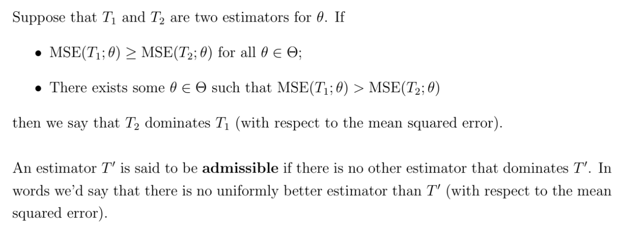
What are dominant and admissible estimators?

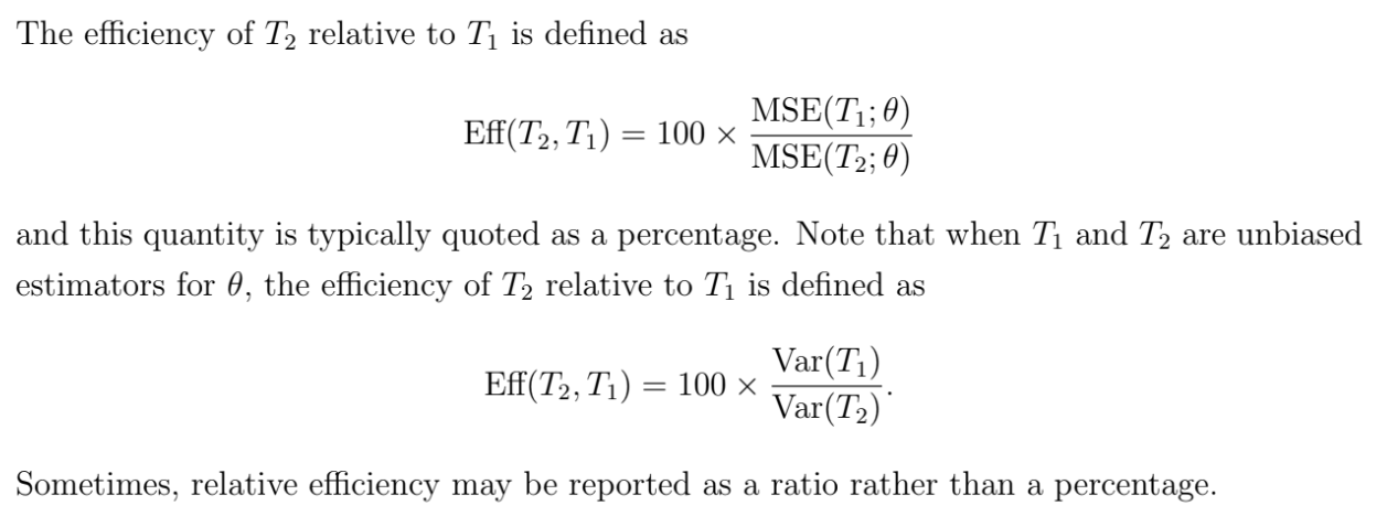
What is the relative efficiency of estimators?

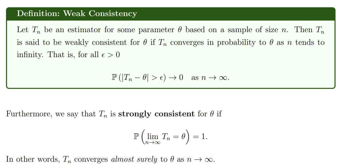
What are weak and strong consistency?

A strongly consistent estimator converges almost surely to $\theta$ as $n\rightarrow\infty$

A weakly consistent estimator only converges in probability

Strong consistency implies weak consistency, but weak consistency does necessarily imply strong consistency

How can we show weak consistency with MSE?

If $MSE(T_{n};\theta)\rightarrow0$ as $n \rightarrow \infty$

then $T_{n}$ is weakly consistent for $\theta$

This property is sufficient but not necessary for weak conssitency

What is the mean of the score function?

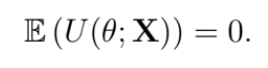
What is the variance of the score function?

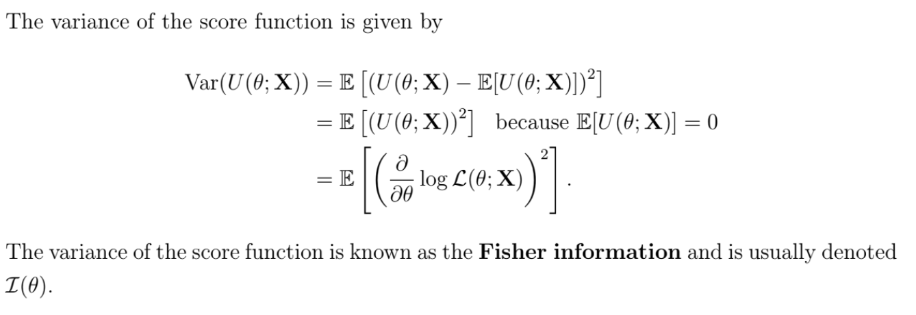
What is the Fisher information?

The Fisher information is the variance of the score function

$$I(\theta) = Var(U(\theta;X)) = E[(\frac{\partial}{\partial \theta}log \mathcal{L} (\theta;X))^{2}]$$

Under certain regularity conditions (i.e. the likelihood function is continuous in $\theta$ and the domain of the density function of X (its support) does not depend on $\theta$), we can show that the Fisher information is also given by

$$I(\theta) = E[-\frac{\partial^{2}}{\partial \theta^{2}} log \mathcal{L}(\theta;X)]$$

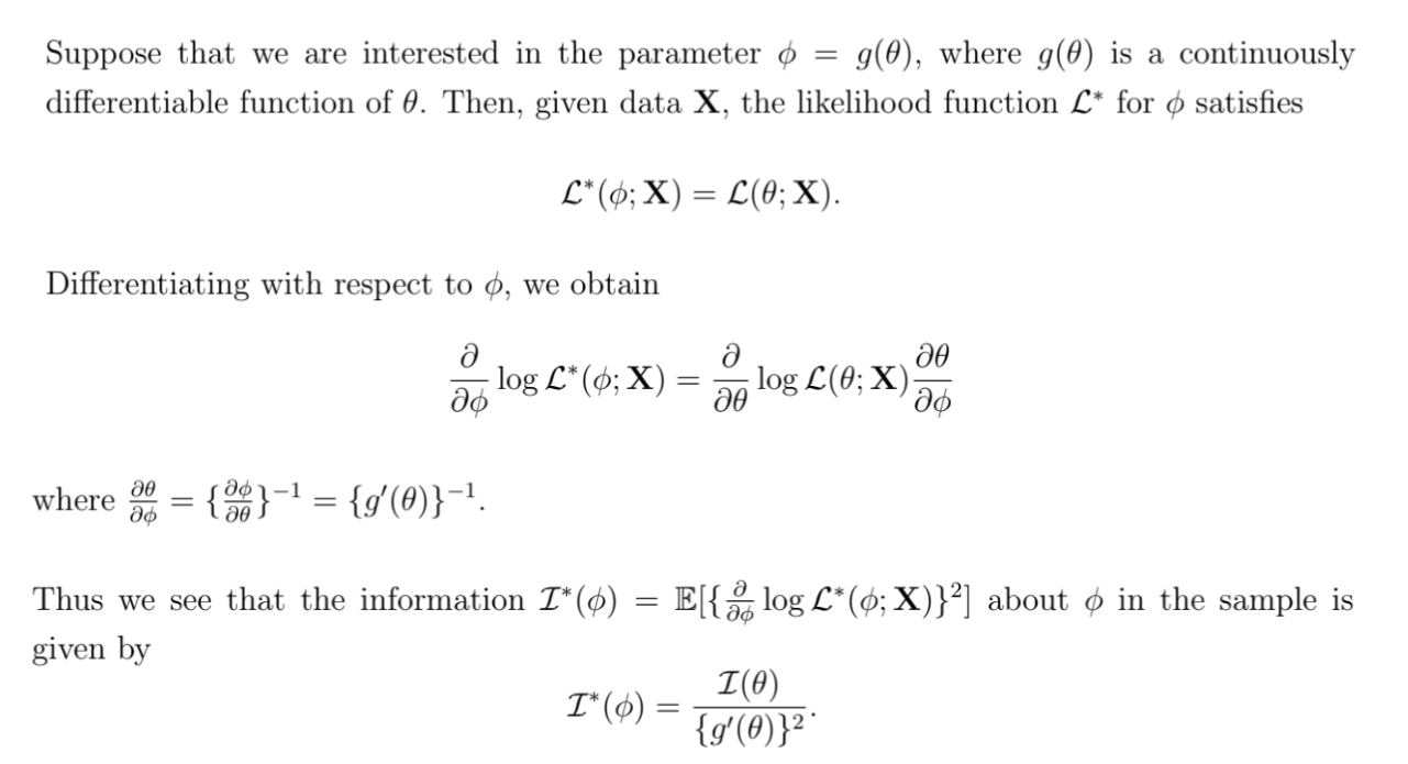
What is the Fisher information of a transformation of $\theta$?

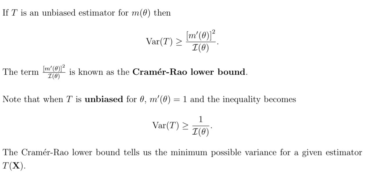
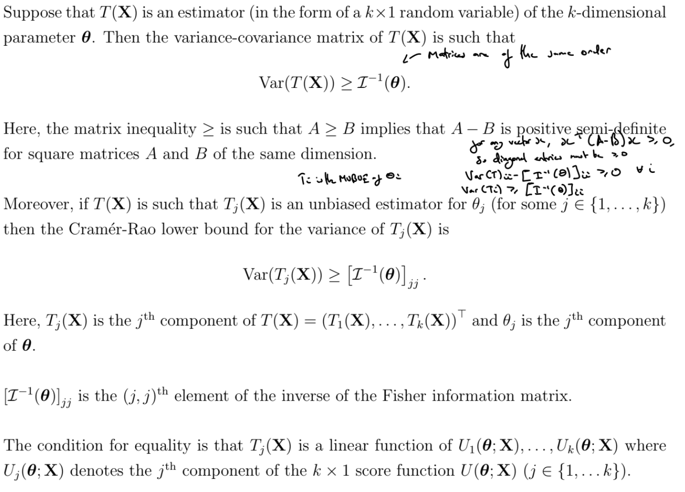
What is the Cramér-Rao lower bound?

Make sure you use $I_n(\theta)$ !!

What is Markov Chain Monte Carlo?

In Bayesian inference, the normalising constant may not be available in closed-form - the integral is intractable.

To produce inferences about the model parameters, we do not need the formula of the posterior distribution, only some summary statistics: posterior mean, posterior median, posterior moments, posterior percentiles, standard deviation, etc. We can calculate these quantities by using a sample from the posterior.

Markov Chain Monte Carlo (MCMC) is a family of methods that can be used to sample from a posterior distribution of interests.

A Markov Chain is a sequence of random draws where each draw only depends on the previous one

Markov chains have 2 important properties

1. Dependence: the Markov property induces a correlation between iterations, which decreases for distant iterations of the chain

2. Equilibrium distribution: the chain stabilises in the long run. After a certain number of iterations, the draws represent (approximate) samples from the equilibrium distribution

Therefore, to sample from a posterior distribution, we need to construct a Markov Chain with an equilibrium distribution equal to the posterior distribution. If we are able to do so, if we run the chain for long enough, we will obtain samples from the posterior distribution

MCMC converges theoretically, however, in some cases it may take a large number of iterations to reach convergence and / or iterations might be highly correlated. Using MCMC samples that have not converged yet may induce bias in the estimators

Look at the traceplots - does it appear that the chain has stabilised?

Auto-correlation plots

Run several chains and see if they converge

What are burn-in and thinning?

The iterations before the Markov Chain has stabilised do not represent approximate samples from the (equilibrium) posterior distribution, so we should discard the first M iterations until the chain looks stable.

An appropriate number of burn-in iterations depends on the choice of the initial point and the proposal distribution.

With narrow proposal distributions it might take a long number of iterations to cover a reasonable region of the target distribution

Wide proposal distributions produce too many bad candidates that will be rejected

With bad initial points, it might take a long number of iterations to reach stability

Iterations are correlated, but this correlation decreases for distant iterations of the chain. To obtain independent samples, we need to sub-sample the chain every K iterations.

The ideal value of K depends on the autocorrelation of the samples

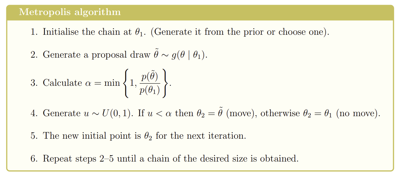
What is the Metropolis algorithm?

Requires

• An initial point,

• A density function proportional to the posterior distribution $p(\theta) = f(x \mid \theta) \pi(\theta) \propto \pi(\theta \mid x)$ ,

• A proposal distribution $g(\theta \mid \eta)$ with $g(\theta \mid \eta) = g(\eta \mid \theta)$. You need to be able to simulate from this distribution. e.g. $\theta\mid\eta\sim Normal(\eta,\sigma^2)$ where $\sigma$ is fixed and controls the length of the steps between iterations

We do not need the normalising constant of the posterior distribution

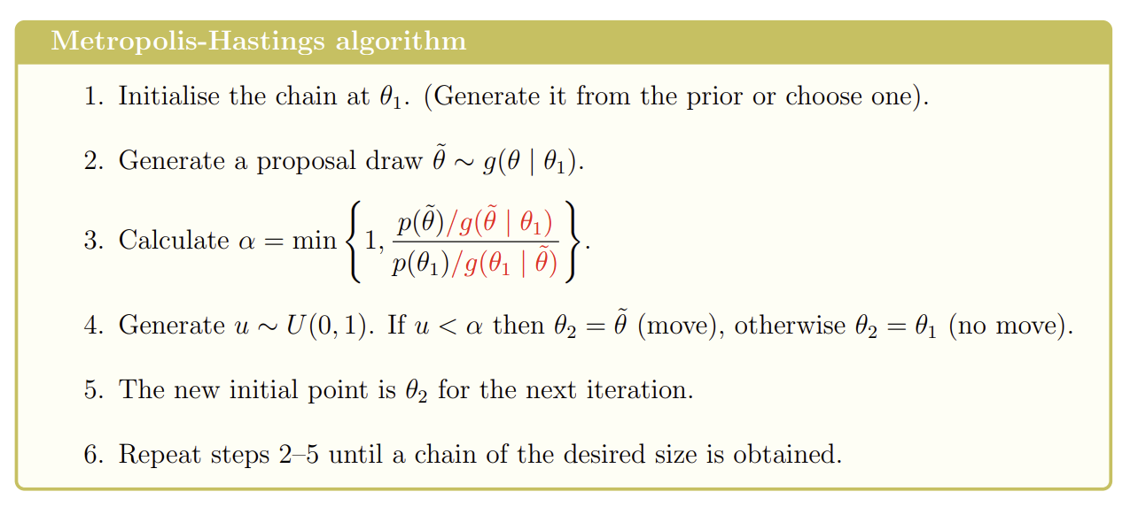
What is the Metropolis-Hastings algorithm?

Requires

• An initial point,

• A density function proportional to the posterior distribution $p(\theta) = f(x \mid \theta) \pi(\theta) \propto \pi(\theta \mid x)$ ,

• A proposal distribution $g(\theta \mid \eta)$. It is not required that $g(\theta \mid \eta) = g(\eta \mid \theta)$. You need to be able to simulate from this distribution

Can easily extend to the multi-parameter case if we have a multivariate proposal distribution (e.g. Multivariate normal)

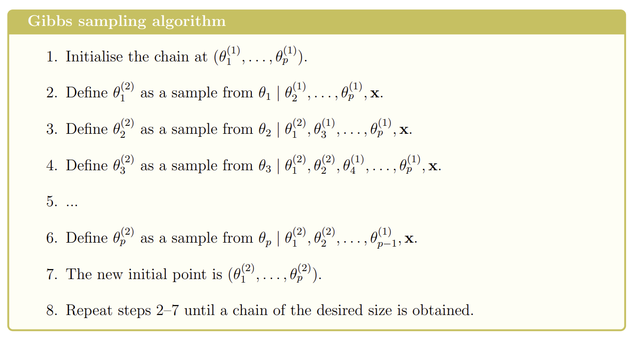
What is the Gibbs sampler?

Used to sample from a posterior distribution of a parameter vector

Requires

• An initial point

• The conditional distributions for each parameter, given the rest of the parameters and the data. You need to be able to sample directly from these distributions

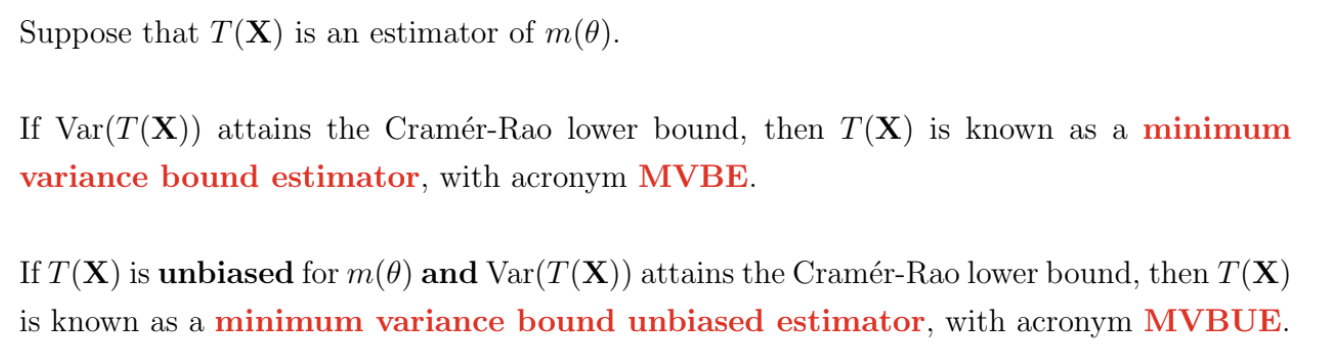
When does the variance of T(X) attain the CR lower bound?

The variance of T(X) attains the CR lower bound if and only if T(X) and $U(\theta;X)$ are linearly related such that

$$U(\theta;X) = A(\theta)(T(X) - m(\theta))$$

The linear form must be as above so that $E[U(\theta;X)]=0$ holds

T(X) is unbiased for $m(\theta)$ and has a variance which attains the CRLB. T is the MVBUE for $m(\theta)$.

Furthermore, it can be shown that $A(\theta)=\frac{I(\theta)}{m^{\prime}(\theta)}$

So

$$U(\theta;X)=\frac{I(\theta)}{m^{\prime}(\theta)}(T(X)-m(\theta))$$

Can easily recover the Fisher information = $A(\theta)m^{\prime}(\theta)$ and the CRLB = $\frac{m^{\prime}(\theta)}{A(\theta)}$

When T(X) is unbiased for $\theta$ then $m(\theta) = \theta$ and $m^{\prime}(\theta)=1$ , so

$$U(\theta;X)=I(\theta)(T(X)-\theta)$$

What are MVBEs and MVBUEs?

What is the score function and variance of the score function for a vector of parameters?

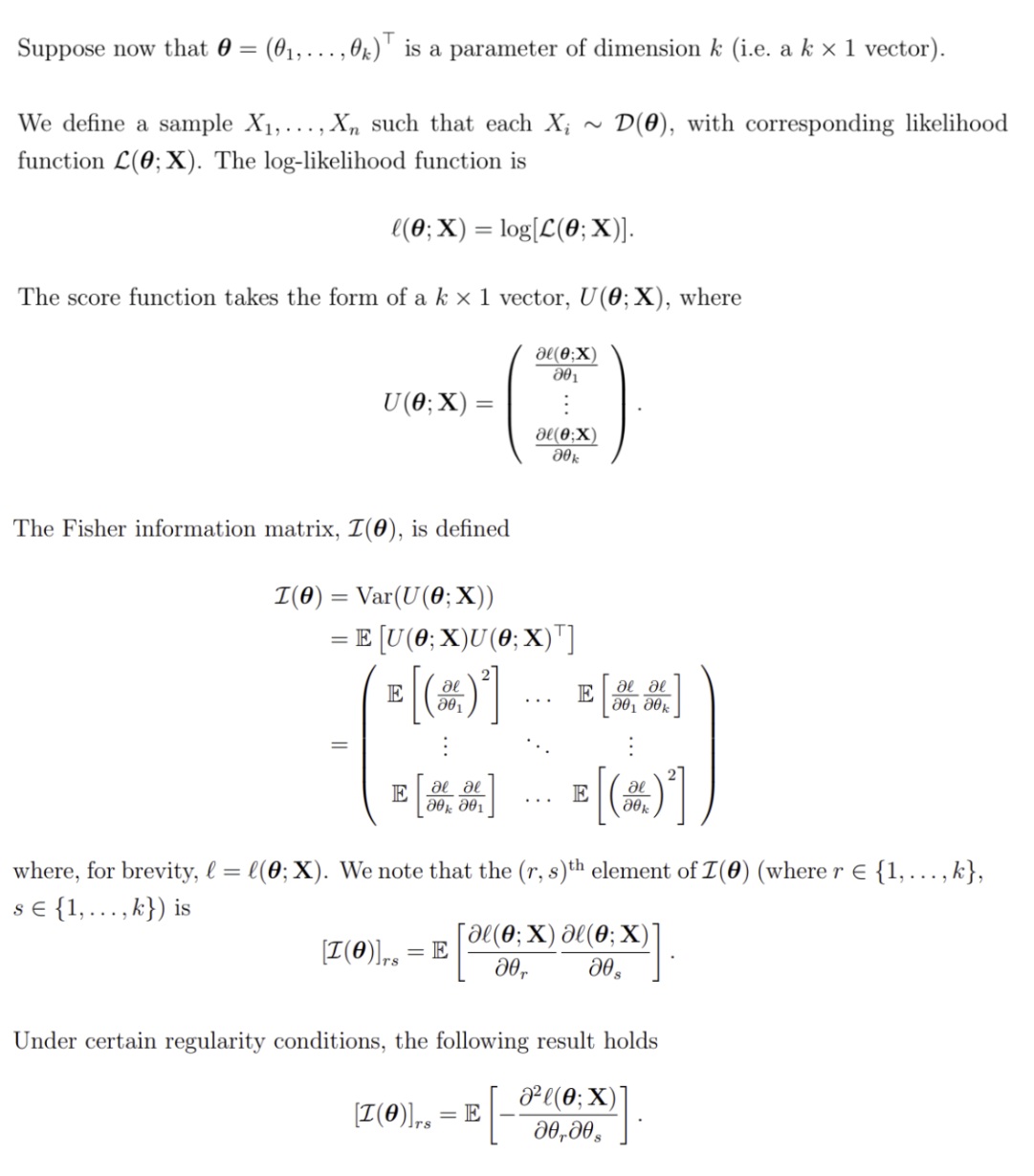
What is the Cramér-Rao lower bound for a k-dimensional parameter?

What is an exponential family of distributions, for one dimensional parameters?

A family of probability distributions with a density / mass function of the form

$$f(x;\theta)=exp\left\lbrace{a(\theta)T(x) + b(\theta) + c(x)}\right\rbrace$$

is said to be an exponential family of distributions

The support of X must not depend on $\theta$

Using the factorisation theorem, we can show that $T(x)$ is sufficient for $\theta$.

Can rearrange to show that the score function is a linear function of $T(x)$, so the variance of $T(x)$ will attain the CRLB.

The likelihood of multiple X is

$$\mathcal{L}(\theta;x)=exp{\left\lbrace a(\theta)T(x)+nb(\theta)+c(x)\right\rbrace}$$

where

$$T(x) = \sum_{i=1}^{n} T(x_{i})$$

and

$$c(x)=\sum_{i=1}^{n}c\left(x_{i}\right)$$

If a distribution is from an exponential family, then sufficient statistics for the distributional parameters are guaranteed to exist, and there exists a conjugate prior distribution for the distributional parameters

Examples of exponential families of distributions are Binomial, Poisson, Exponential, Normal, Gamma, Beta, etc.

What is an exponential family of distributions, for k-dimensional parameters?

Suppose now that $\theta$ is k-dimensional

A family of probability distributions is an exponential family if

$$f(x;\theta)=exp{\left\lbrace\sum_{r=1}^{k}a_{r}(\theta)T_{r}(x)+b(\theta)+c(x)\right\rbrace}$$

As in the one-dimensional case, the support of X must not depend on $\theta$

Using the factorisation theorem, we can show that $T_1\left(x),...,T_{k}\left(x\right)\right.$ are jointly sufficient for $\theta$

Where the number of jointly sufficient statistics is equal to the dimension of $\theta$ , $T_1\left(x),...,T_{k}\left(x\right)\right.$ may be expressed as linear functions of $U_{j}(\theta;X)$ and so estimators that are linear functions of $T_1\left(x),...,T_{k}\left(x\right)\right.$will have variances than attain the CRLB

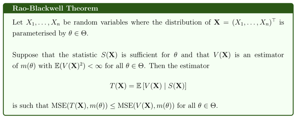
What is the Rao-Blackwell theorem?

We will have equality if and only if $V(X)$ is a function of X only through $S(X)$.

If $V(X)$ is unbiased for $m(\theta)$, then $T(X)$ is also unbiased for $m(\theta)$ and $Var(T(X)) \leq Var(V(X))$

$T(X)$ does not depend on $\theta$ because the distribution of X, conditional on $S(X)$ does not depend on $\theta$ (since $S(X)$ is sufficient for $\theta$)

Essentially: if we take an estimator $V(X)$ for $m(\theta)$ and then take the expectation of $V(X)$ conditional on $S(X)$, where $S(X)$ is a sufficient statistic for $\theta$, then we will obtain an estimator with mean squared error that is less than or equal to that of the original estimator $V(X)$.

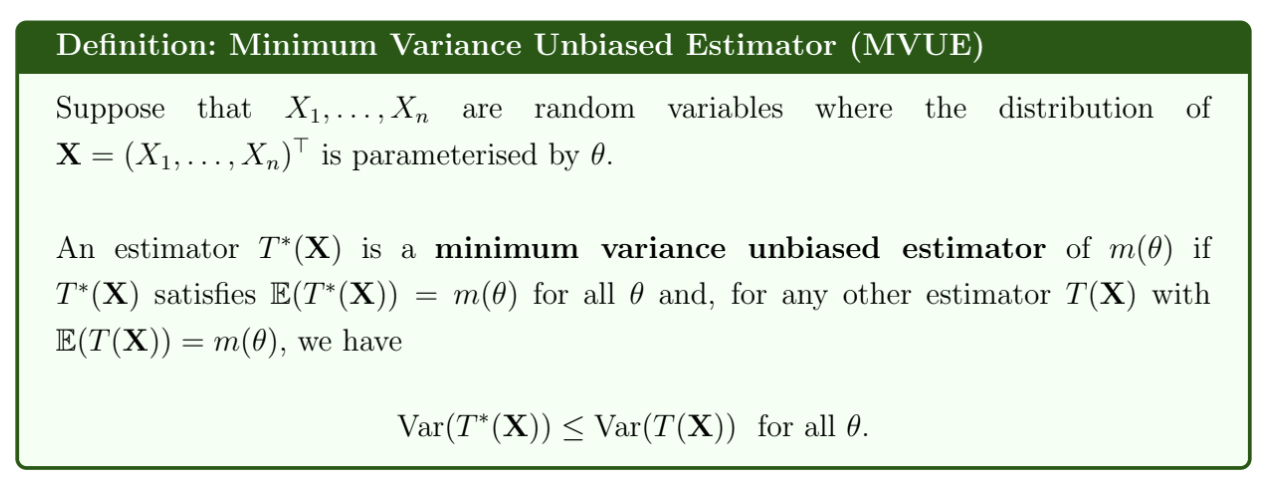
What is a Minimum Variance Unbiased Estimator?

The variance may not attain the CRLB - if it does, it is a minimum variance bound unbiased estimator

The minimum variance unbiased estimator is unique

If $T(X)$ is the MVUE of $m(\theta)$, then $T(X)$ must be uncorrelated with all unbiased estimators of 0. If an estimator is correlated with a random noise, then it can be improved.

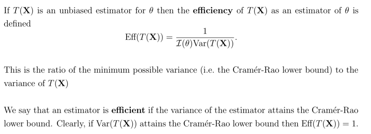
What is the efficiency of an estimator?

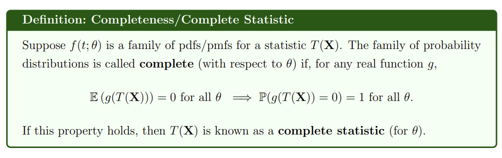
What is completeness / a complete statistic?

If a statistic has a distribution that belongs to the exponential family of distributions, then the statistic is complete with respect to the unknown distributional parameters

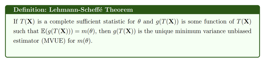
What is the Lehmann-Scheffé theorem?

What are the general properties of maximum likelihood estimators?

A maximum likelihood estimator is necessarily a function of a minimal sufficient statistic

If an estimator, T(X), exists such that T(X) is the MVBUE of an unknown parameter $\theta$, then T(X) is the maximum likelihood estimator of $\theta$

If $\hat{\theta}$ is the maximum likelihood estimate of $\theta$, then the maximum likelihood estimate of $g(\theta)$ is $g(\hat{\theta})$. More generally, in the multiparameter case, if we re-parameterise the likelihood function using functions of the original parameters, then the maximum likelihood estimates of our new parameters are the corresponding functions of the maximum likelihood estimates of our original parameters.

What are the asymptotic properties of maximum likelihood estimators?

Under the weak regularity conditions that

1. The likelihood function $\mathcal{L}(\theta; X)$ is continuous in $\theta$

2. The density / mass function $f(x;\theta)$ is such that for all $x$ where f(x;\theta) > 0, $\frac{\partial}{\partial \theta} logf(x;\theta)$ exists and is finite. In other words, the log-likelihood function is differentiable.

3. The order of differentiation with respect to $\theta$ and integration over the sample space $\mathcal{X}$ may be reversed. This is satisfied when the support of $f(x;\theta)$ does not depend on $\theta$.

Then the following properties hold:

1. The maximum likelihood estimator is a strongly consistent estimator of $\theta$ $\mathbb{P}\left(\lim_{n\rightarrow\infty}T_{n}\left(X\right)=\theta\right)=1$. It follows that the MLE is asymptotically unbiased.

2. The maximum likelihood estimator is asymptotically efficient: $\lim_{n\rightarrow\infty}Var(T_{n}(X))=\frac{1}{I\left(\theta\right)}$ . If the sample size is large, the variance of the MLE is approximately equal to the CRLB. Since the MLE is also asymptotically unbiased, it follows that for large samples, the MLE is approximately the MVBUE of $\theta$

3. The maximum likelihood estimator is asymptotically normally distributed: $T_{n}(X)\sim N(\theta,\frac{1}{I(\theta)})$ for large n: $\sqrt{n}(\hat{\theta}-\theta)\stackrel{d}{\sim}N\left(0,\frac{1}{I_1(\theta)}\right)$

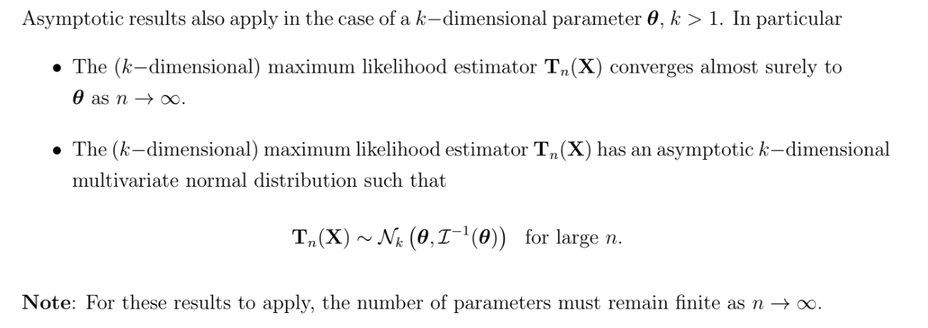
What are the asymptotic properties of the maximum likelihood estimator of a k-dimensional parameter?

How do we choose a prior distribution?

We can specify a personal prior, corresponding with our view of the uncertainty about a parameter value, based on expert opinion or deep subject knowledge. Two observers might have two very different personal priors.

If we don’t want to use a personal prior, we can choose a prior that is quite vague, such as a uniform prior or a Jeffreys’ prior

What is a uniform prior?

A uniform or flat prior is a prior distribution where each possible value of $\theta$ is, a priori, equally likely

Can be either a discrete or continuous uniform distribution

May be an improper prior, e.g. if $\theta \in (-\infty,\infty)$

What is an improper prior?

Can obtain a proper posterior from an improper prior

What is Jeffreys’ prior?

Jeffreys’ prior is

$$\pi(\theta)\propto\sqrt{I{_1\left(\theta\right)}}$$

Note that $I_1(\theta)$ is the Fisher information of a single observation - not dependent on n!

Jeffreys’ prior is invariant under re-parameterisation of $\theta$, i.e.

$$\pi(\theta)\propto\sqrt{I_1(\theta)}\iff\pi(g(\theta))\propto\sqrt{I_1(g(\theta))}$$

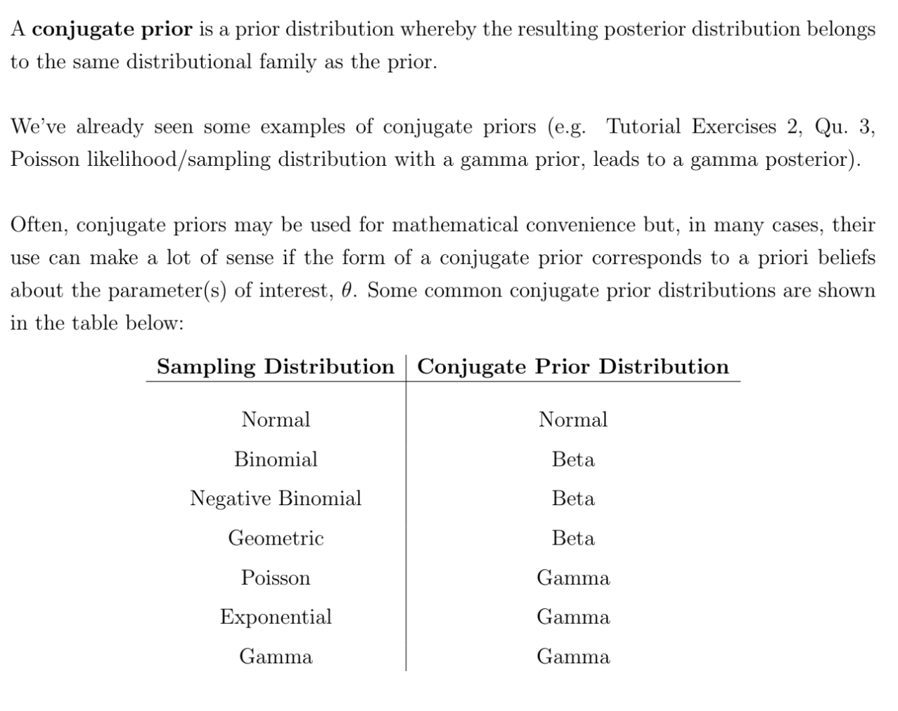
What is a conjugate prior?

A conjugate prior distribution is a prior distribution where, when combined with a given likelihood function, the posterior distribution belongs to the same family as the prior

How do we carry out Bayesian point estimation?

Let the loss incurred in using t(x) to estimate $\theta$ be the loss function $L(\theta, t(x))$

The Bayes estimate of $\theta$, denoted $\theta$* is the value t = t(x) that minimises the posterior expected loss

$$\mathbb{E}_{\theta \mid x}[L(\theta, t)] = \int_{\Theta} L(\theta, t) \pi (\theta \mid x) d\theta$$

Notably, under quadratic error loss, the loss function is $L(\theta, t) = (\theta - t)^{2}$ and the Bayes’ estimate is the posterior mean

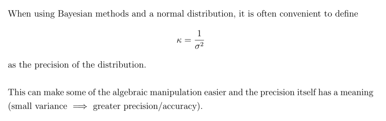
What is the precision of a normal distribution?

What are simple and composite hypotheses?

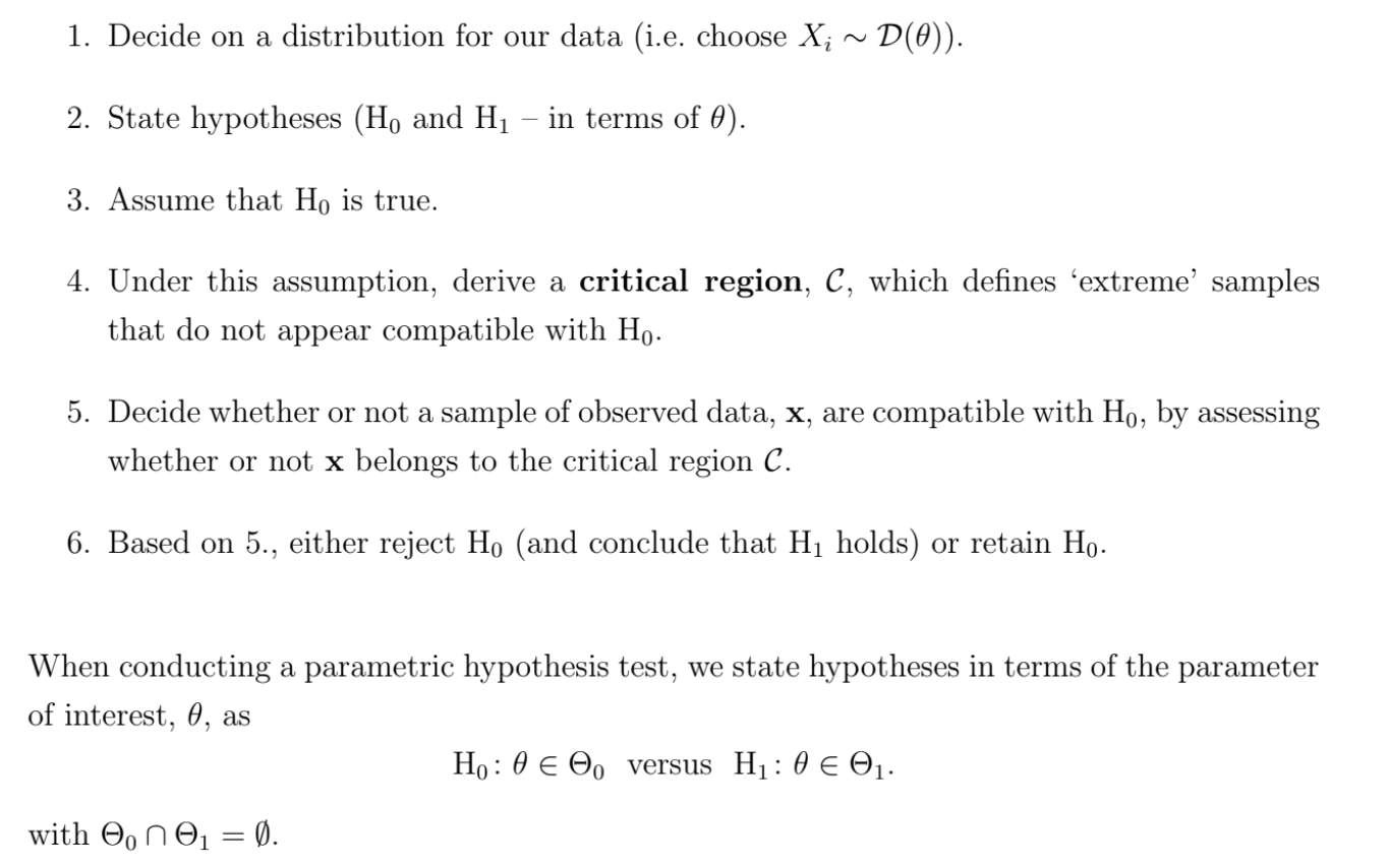
A hypothesis about $\theta$ can be expressed as

$$H_{0}: \theta \in \Theta_{0}$$

If $\Theta_{0}$ consists of a single value, then the corresponding hypothesis is a simple hypothesis.

e.g. $H_{0}: \theta = 0$

Otherwise, a hypothesis is a composite hypothesis

e.g. H_0:\theta>0

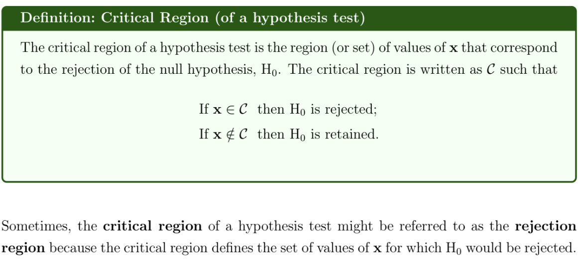
What is the critical region of a hypothesis test?

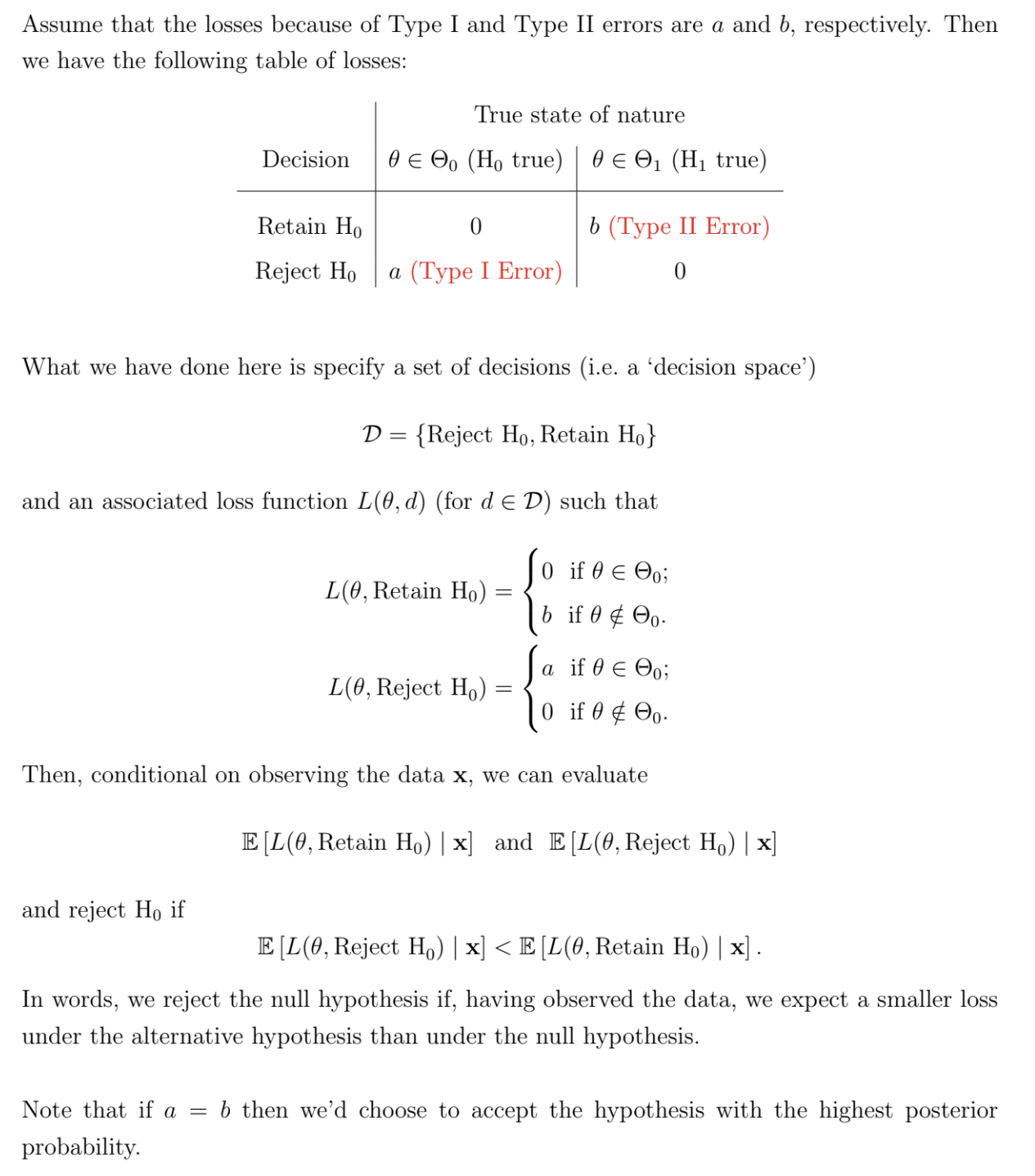
What are type I and type II errors, and the size and power of a hypothesis test?

There are two possible errors that could be made in a hypothesis test

Type I error: Reject $H_0$ when $H_0$ is true (a false positive)

Type II error: Retain $H_0$ when $H_0$ is false (a false negative)

The probability of a Type I error is

$$\alpha(\theta)=P(\text{Type I error})=P(X\in C\mid\theta\in\Theta_0)$$

The probability of a Type II error is

$$\beta(\theta) = P(\text{Type II error)} = P(X \in C \mid \theta \not\in \Theta_0)$$

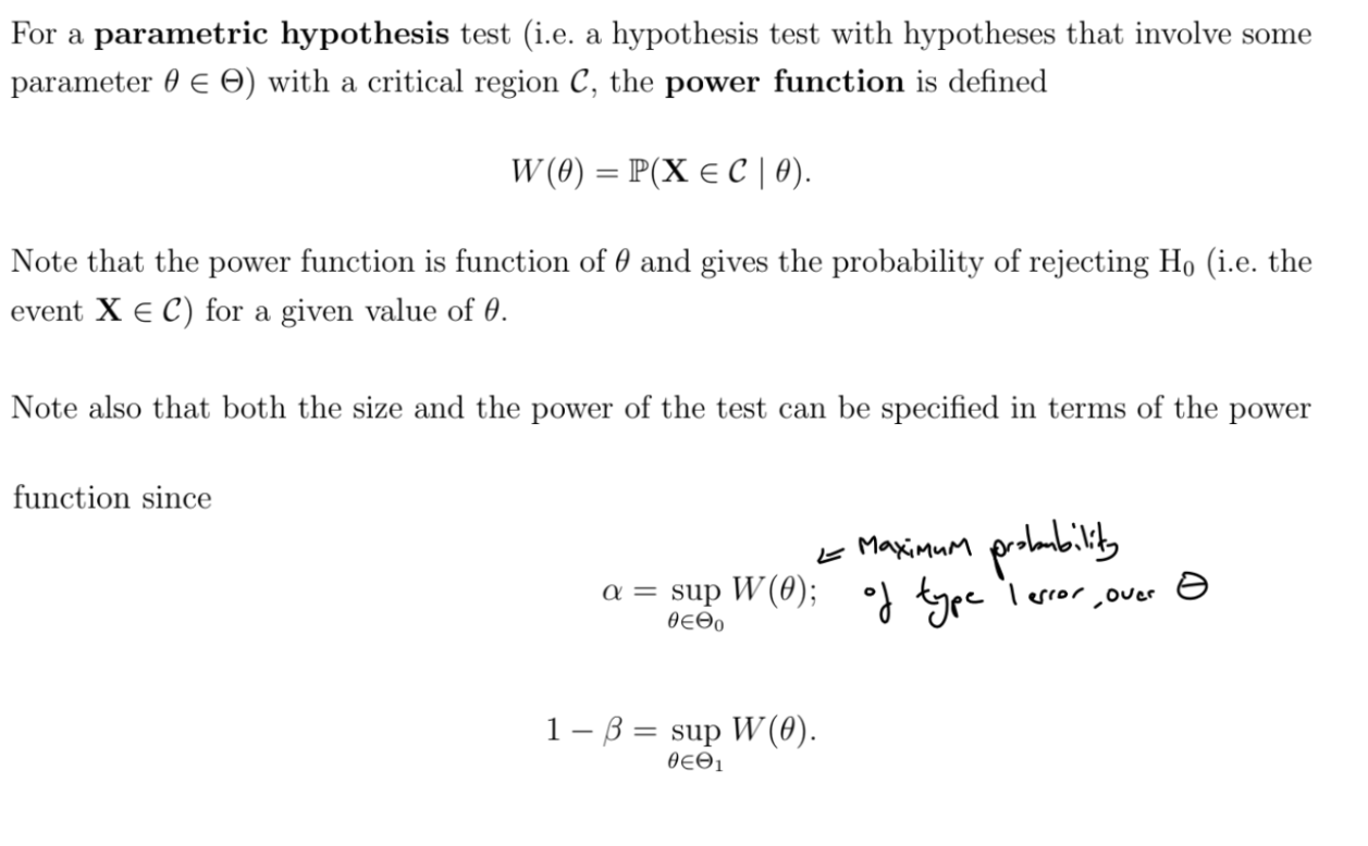
The size / significance level of a hypothesis test is

$$\alpha=sup_{\theta\in\Theta_0}\alpha(\theta)=sup_{\theta\in\Theta_0}P(X\in C\mid\theta\in\Theta_0)$$

The power of a hypothesis test is

$$1-\beta(\theta) = 1- P(\text{Type II error)} = 1-P(X \in C \mid \theta \not\in \Theta_0)$$

What is a P-value?

For a two-sided test,

p=P\left(\left\vert{T(X)}\right\vert>t(x\right)\mid H_0)

For one sided tests,

p = P(T(X) > t(x) \mid H_0) if we reject $H_0$ when $t(x)$ is large

p = P(T(X) < t(x) \mid H_0) if we reject $H_0$ when $t(x)$ is small

In words, the P-value is the probability of observing a sample $x$ or a more ‘extreme’ sample under the assumption that $H_0$ is true

Conventionally,

p < 0.01 might be regarded as strong evidence against $H_0$

p < 0.05 might be regarded as sufficient evidence against $H_0$

These notions depend on the problem being studied and the consequences of a type I error

What are the steps of a parametric hypothesis test?

What is the power function?

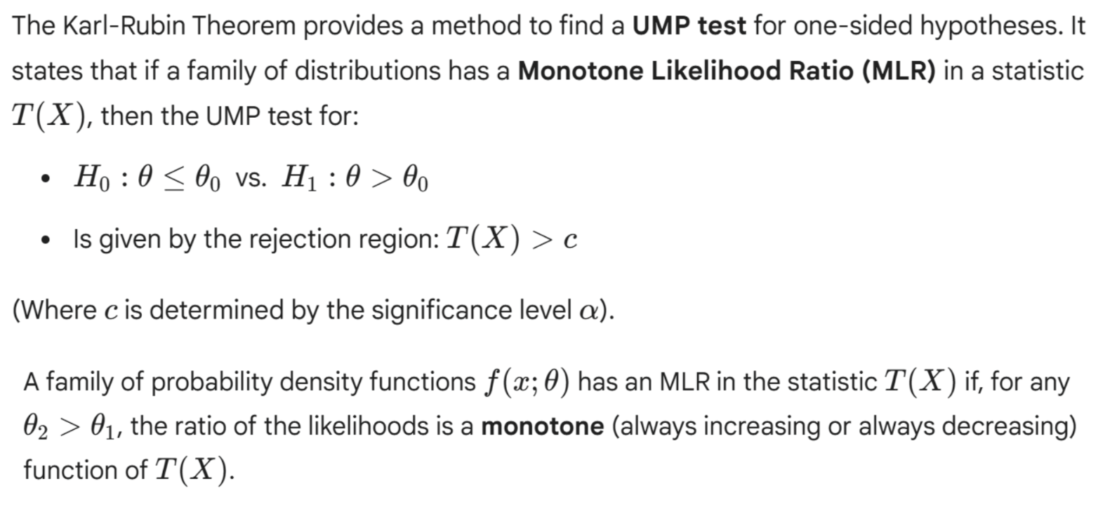
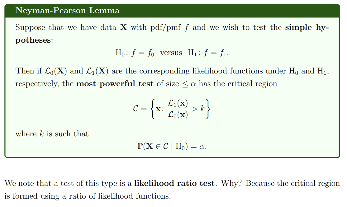
What is the Neyman-Pearson Lemma?

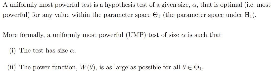
What is a uniformly most powerful test?

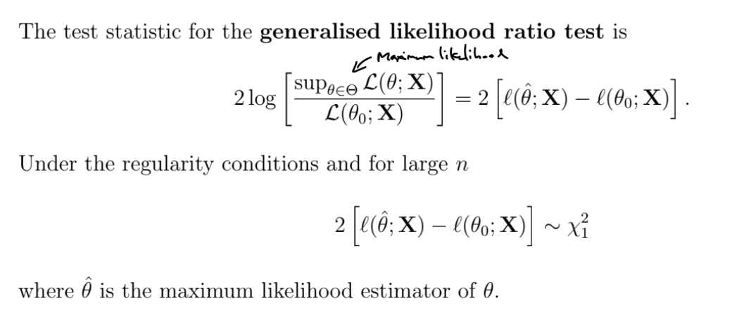
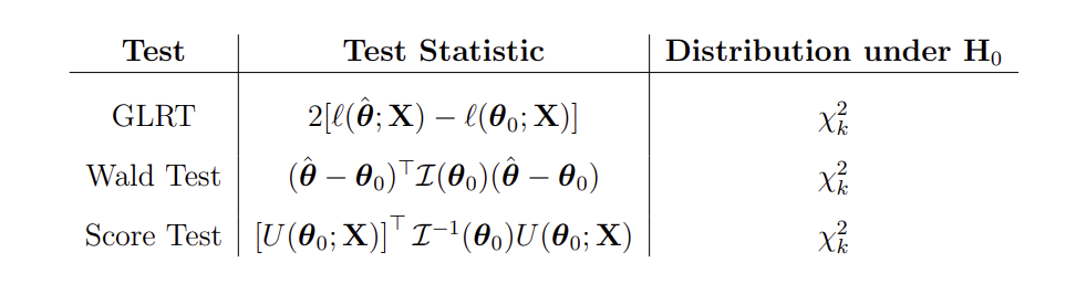
What is the generalised likelihood ratio test?

Testing the null hypothesis $H_0:\theta=\theta_0$ against the general alternative $H_1: \theta \not= \theta_0$

Calculate sample statistic and compare to the critical value of the $\chi_1^2$ distribution

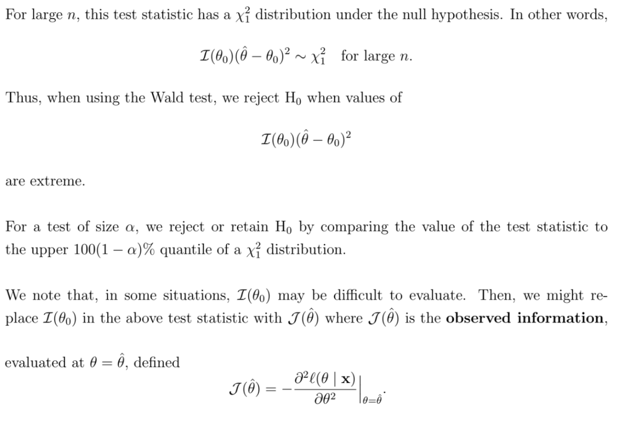
What is the Wald test?

Testing the null hypothesis $H_0:\theta=\theta_0$ against the general alternative $H_1: \theta \not= \theta_0$

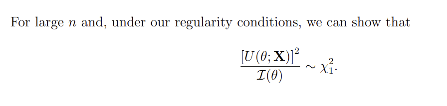
What is the Score test?

Testing the null hypothesis $H_0:\theta=\theta_0$ against the general alternative $H_1: \theta \not= \theta_0$

Calculate sample statistic and compare to the critical value of the $\chi_1^2$ distribution

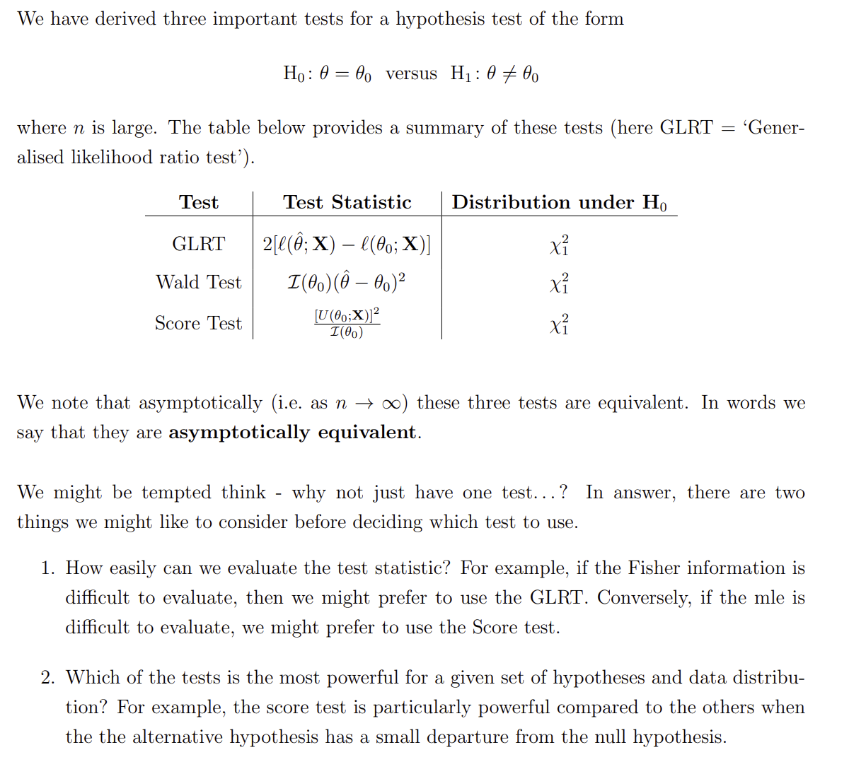
How do the Generalised Likelihood Ratio Test, Wald Test and Score Test compare?

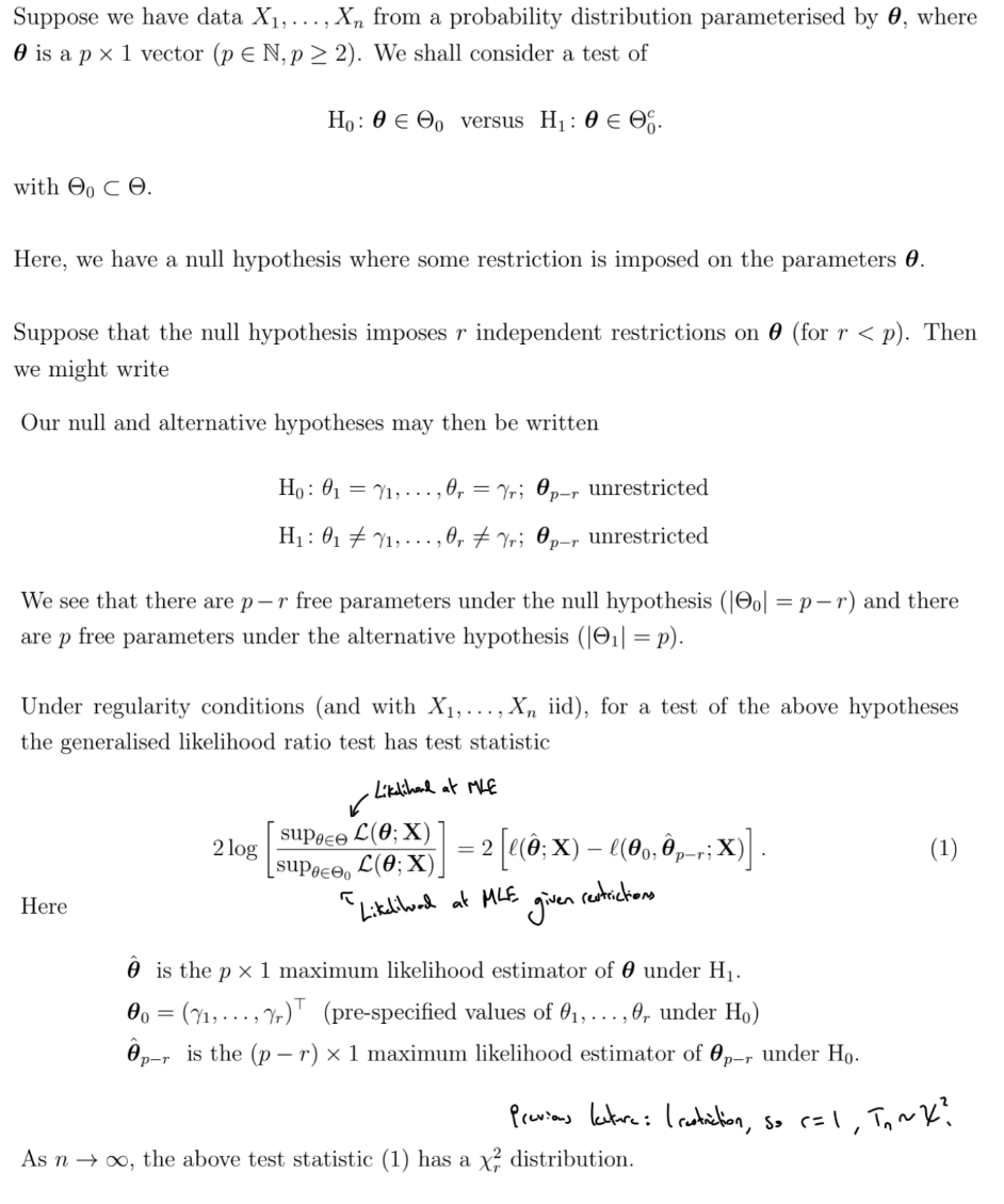
What are the multi-parameter Generalised Likelihood Ratio Test, Wald Test and Score Test?

If $\theta$ is a $k \times 1$ vector

If our model has many parameters, we should do a single test, rather than one parameter tests on each parameter. From the 2nd test onwards, the results depend on whether the previous tests were accurate - so Type I error is inflated

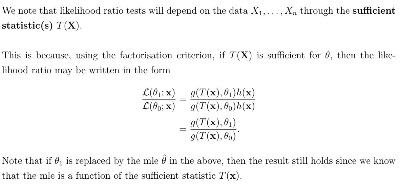
What is the relationship between likelihood ratio tests and sufficiency?

What is a further generalised likelihood ratio test?

If this likelihood ratio can be used to form a test where the distribution of a test statistic is known exactly, then we would use this instead of the asymptotic chi-squared approximation - e.g. t-tests and F-tests

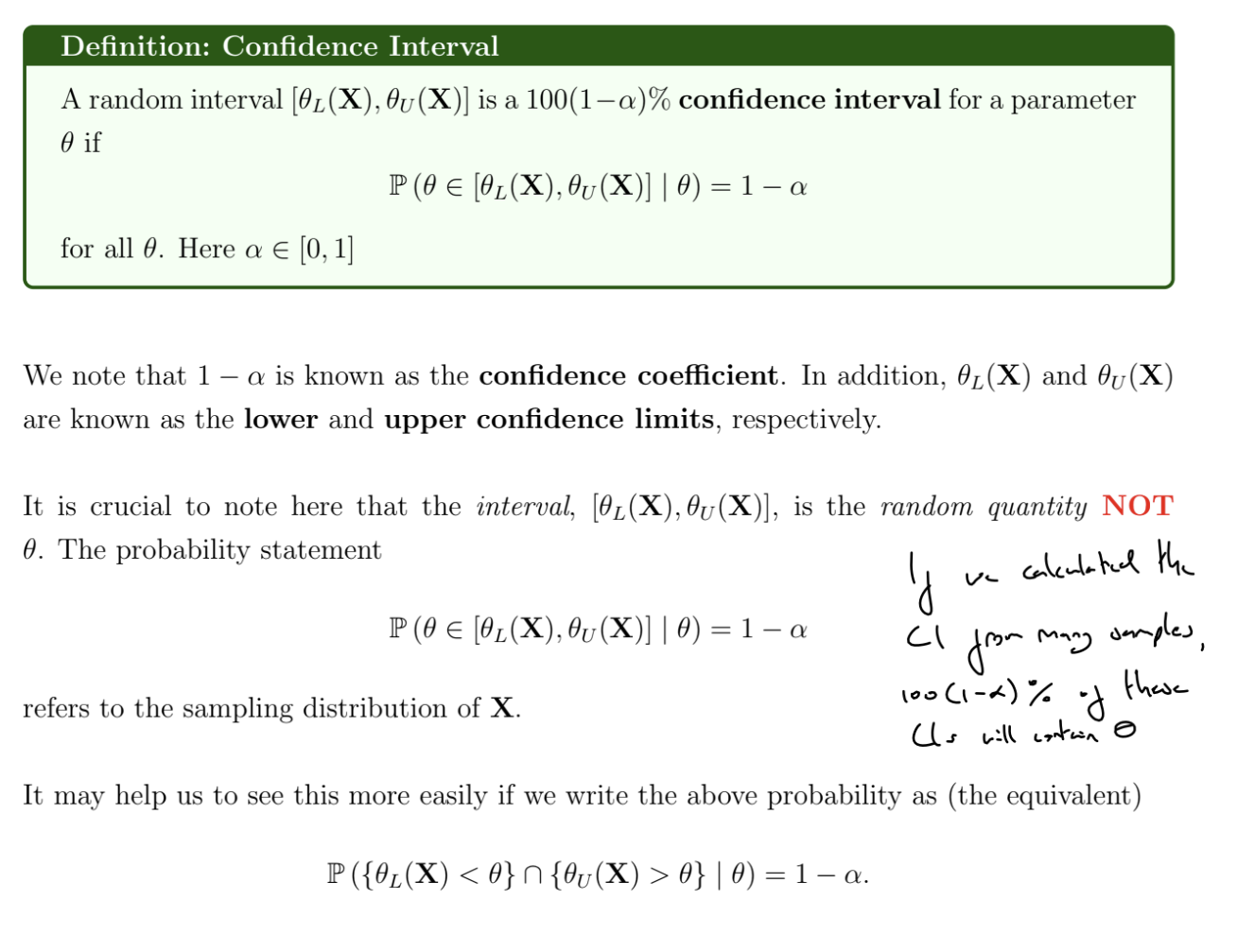
What is a confidence interval?

Can obtain a confidence interval for $\theta$ by using the distribution of an unbiased estimator of $\theta$, e.g. $\bar{X}$ for $\mu$

There are infinitely many valid $100(1-\alpha)\%$ confidence intervals.

We may want the tails to have equal probability (central confidence interval) or the interval to be as narrow as possible

What is a pivotal quantity?

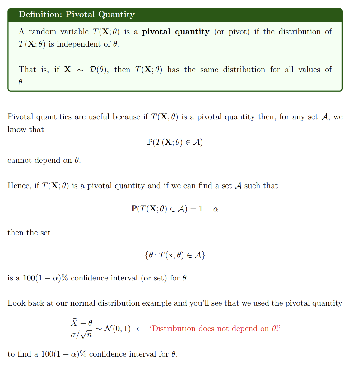
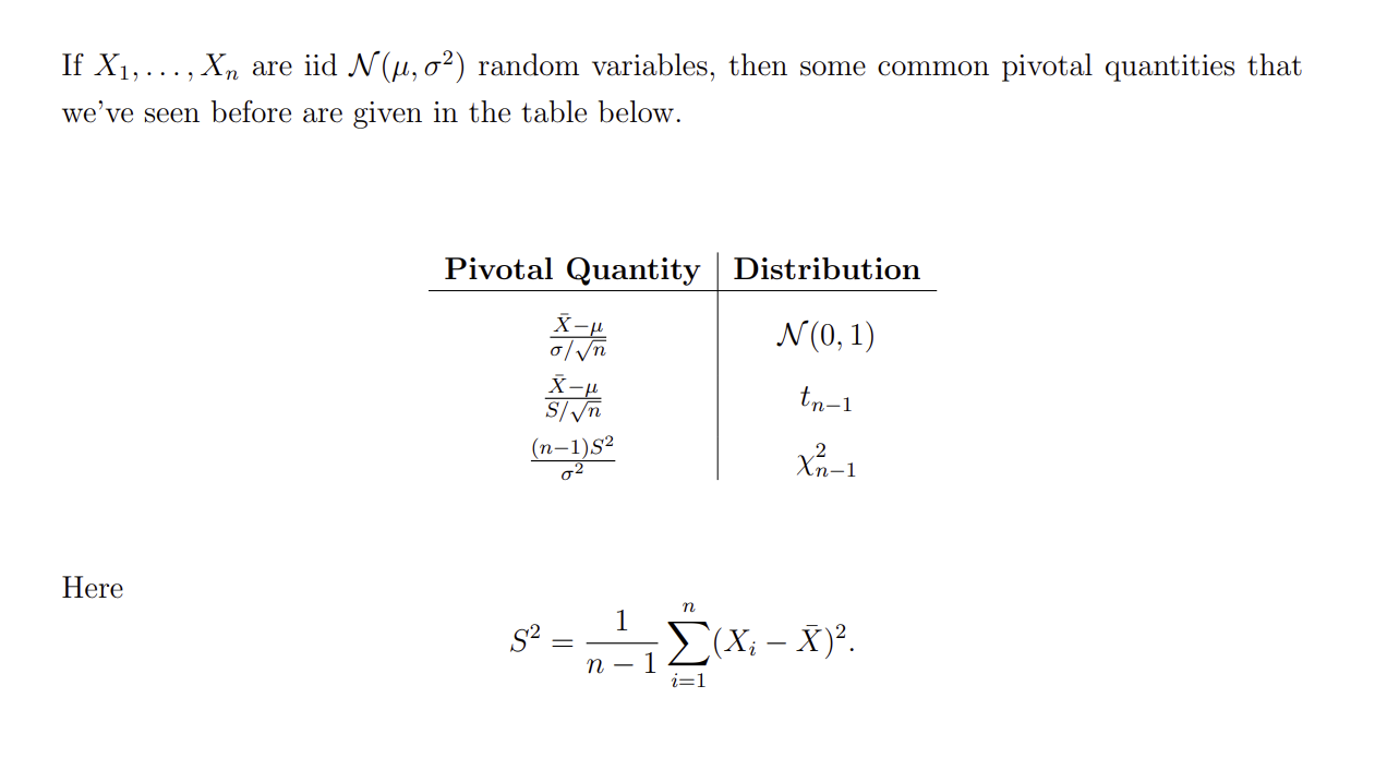
What are common pivotal quantities for the normal distribution?

What is the relationship between confidence intervals and hypothesis testing?

There is a direct relationship between a $100(1-\alpha)\%$ confidence interval and a size $\alpha$ hypothesis test. If the sample $x$ would result in the null hypothesis $H_0: \theta = \theta_0$ being retained in a test of size $\alpha$, then $\theta_0$ lies within the corresponding $100(1-\alpha)\%$ confidence interval constructed using $x$, and vice versa.

$$x \in A(\theta_0) \iff \theta_0 \in B(x)$$

where A is the acceptance region and B is the confidence interval

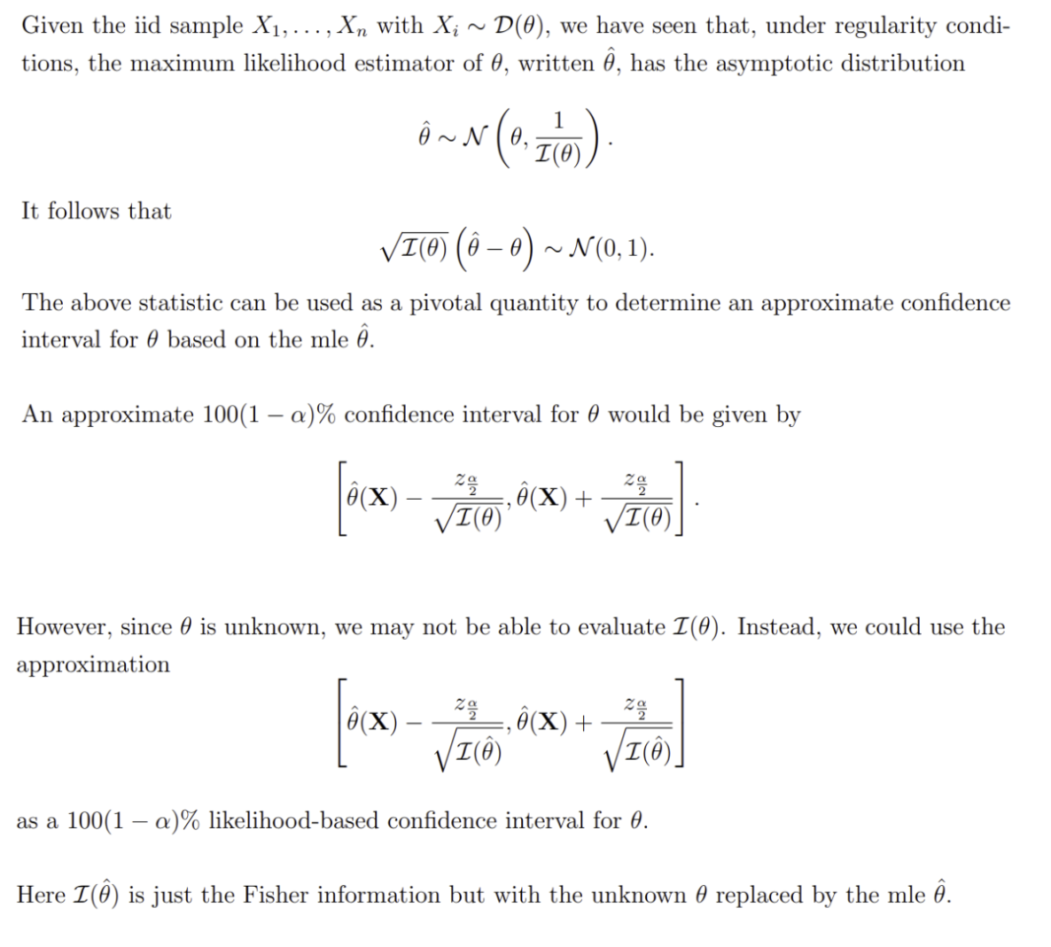
How can we construct a confidence interval based on the maximum likelihood estimator?

This is an approximate confidence interval

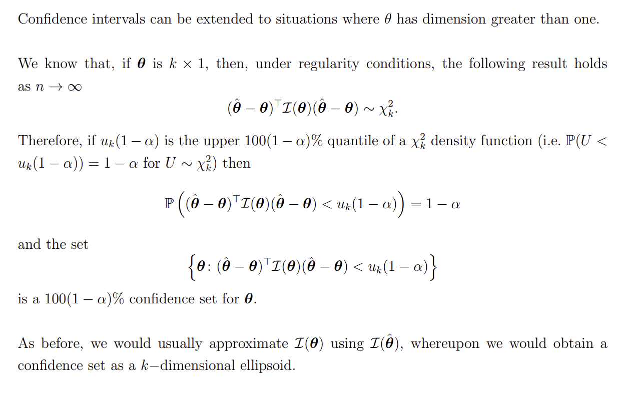
What is a confidence region / set?

How can we construct a confidence interval using the probability integral transform?

Suppose that we have $X_1, …, X_n$ with $X \sim \mathcal{D}(\theta)$, where $T(X)$ is sufficient for $\theta$, and $T(X)$ is a continuous random variable with CDF:

$$F(t, \theta) = P(T(x) \le t \mid \theta)$$

If we define the random variable

$$U(T(X), \theta) = F(T(X), \theta)$$

then $U(T(X), \theta) \sim U[0,1]$, and hence $U(T(X), \theta)$ is a pivotal quantity

Since $T(X)$ is a continuous random variable and $F(t, \theta)$ is a strictly increasing function of $t$, then $F^{-1}$ exists

Because $U(T(X), \theta)$ is a pivotal quantity and the CDF of U is known, we can re-arrange the CDF to obtain a confidence interval

How do we carry out Bayesian Hypothesis Testing?

For simple hypotheses, if the losses are constant (do not depend on $\theta$) we can see that the Bayesian hypothesis test procedure results in a likelihood ratio test

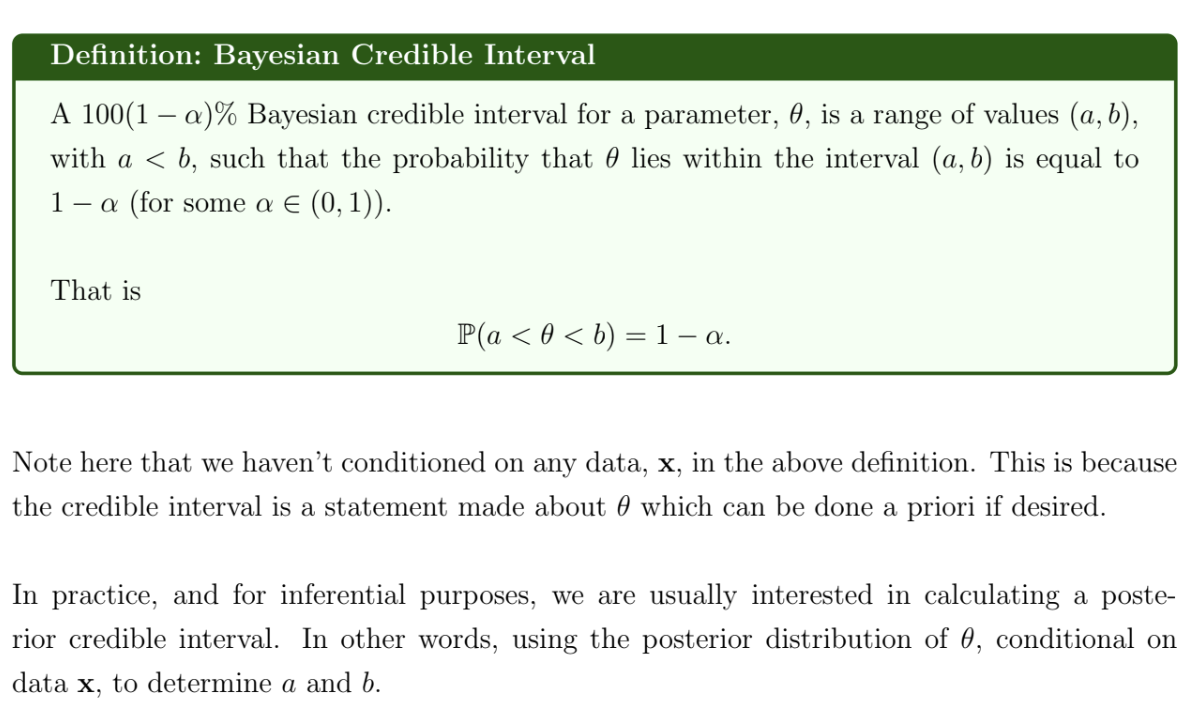
What is a Bayesian credible region?

There are many possible choices for a $100(1-\alpha)\%$ confidence interval. We might choose the most narrow interval, or the central credible interval.

If $X_1,…,X_n$ are independent and identically distributed and our usual regularity conditions are satisfied, when n is large, our posterior distribution is approximately

$$\theta\mid x \sim N(\hat{\theta},\frac{1}{I\left(\hat{\theta}\right)})$$

We can use this to obtain a credible region when n is large

What does $\dot\sim$ mean?

Approximately distributed

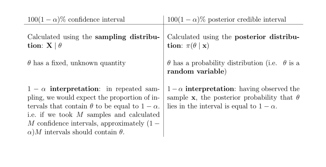
What are the differences between confidence intervals and credible intervals?

What is the relationship between $I_1(\theta)$ and $I_n(\theta)$?

If the samples are iid

$$I_{n}(\theta)=E[-\frac{\partial^{2}}{\partial\theta^{2}}\log f(X;\theta)]=E[-\sum_{i=1}^{n}\frac{\partial^{2}}{\partial\theta^{2}}\log f(x_i;\theta)]$$

$$=\sum_{i=1}^{n}E[-\frac{\partial^{2}}{\partial\theta^{2}}\log f(x_{i};\theta)]=\sum_{i=1}^{n}I_1(\theta)=nI_1\left(\theta\right)$$

What is the Karl-Rubin theorem? (No longer in course)