michalemas math part II

delta function property (the important one)

∫ δ(x − ξ)f(x)dx = f(ξ) (∞ to −∞)

differential operator L

L = d²/dx² + p(x) d/dx + q(x)

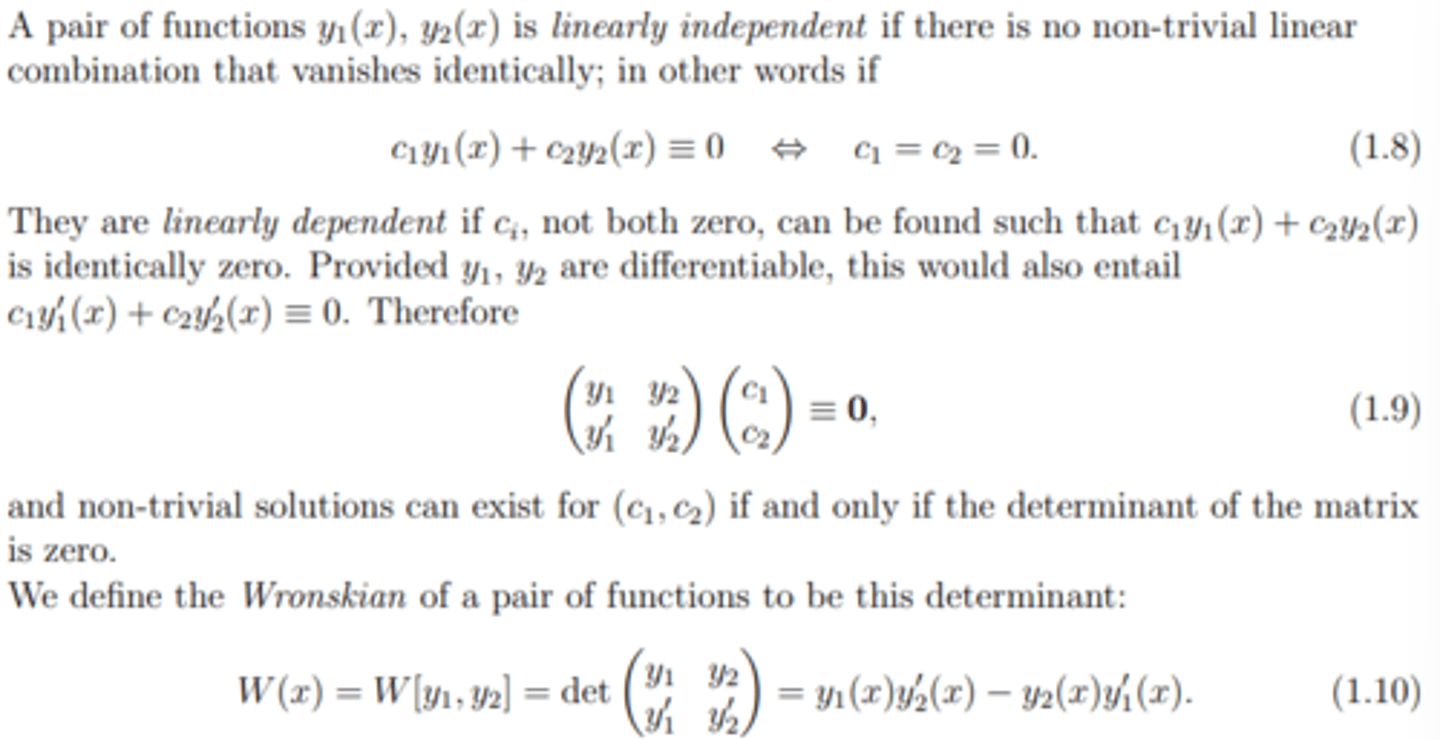
The Wronskian

W = y₁y₂' -y₂y₁'

y₁, y₂ are solutions to an ODE and are independent for W≠0

Two Properties Green's Functions that allow to solve the DEs:

at the boundary:

∂G⁺/∂x - ∂G⁻/∂x =1

G⁺= G⁻

solution for Ly(x) = f(x) using G(x; ζ)

y(x) = ∫ G(x; ζ)f(ζ) dζ from a to b (the given boundry points)

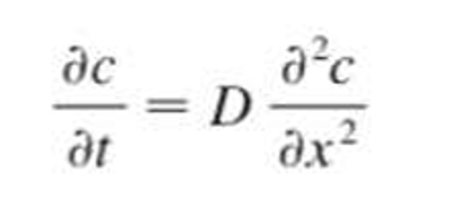
steps for solving seperable linear PDEs

(i) inhomogeneous equation, find a particular solution.

(ii) Seek separable solutions to the homogeneous equation.

(iii) In the case of inhomogeneous boundary conditions (non constant - eg one wall is cold, one hot in the end) we split the solution into two: steady state and homogenous solution. Find the steady-state solution by guessing (eg linear gradient between C1 and C2 along x results in (C2-C1)/L x).

(iv) solve the homogeneous case (zero at the boundaries). using separable function. The BC will determine wether λ>,<, = 0. Find the eigenvalues, eg kₙ = nπ/L and the eigenfunctions Xₙ = Γₙ sin(kₙ x). the solution is the sum of eigenfunctions from n=1 to ∞.

(vi) add the solutions from (i) - (iv). Determine unknown constants using the boundary conditions.

note: The idea is to handle sources (particular integral), handle boundary conditions (if they're inhomogeneous) , then solve the homogeneous "leftover" problem using separation of variables. So the most complicated it will get is y(x,t)=v(x,t)+w(x)+p(x,t).

connection between a transformation matrix and the transformed basis

Each column tells you where one original basis vector ends up after the transformation. The j-th column is the transformed version of the j-th basis vector

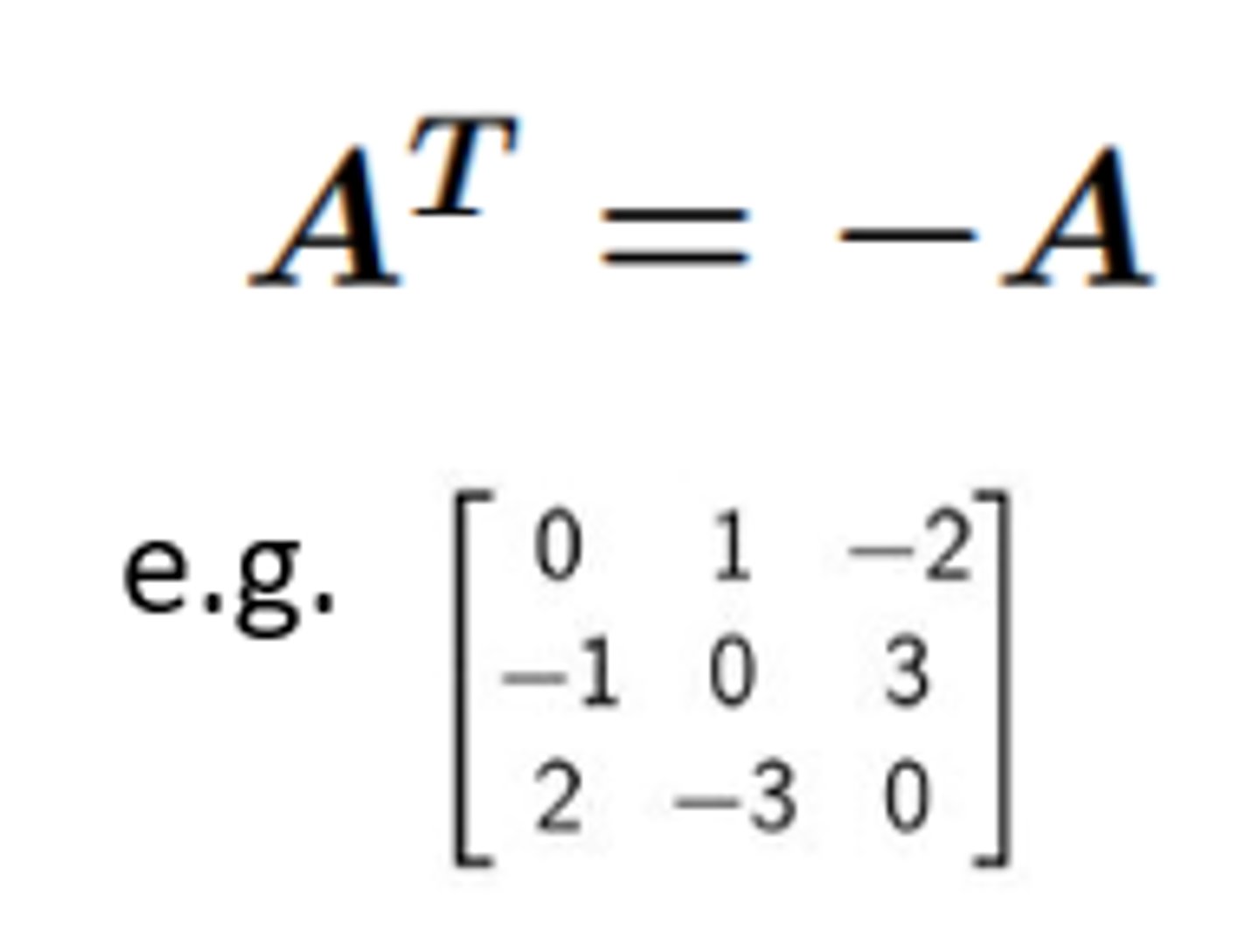
symmetric and antisymmetric matrices

A^T = A

A^T = -A

definitions and properties of:

Normal matrices

Orthogonal matrices

unitary matrices

normal matrix: AA† = A†A

Orthogonal matrix: Q⊤Q=QQ⊤=I

Unitary matrix: U*U=UU* = I

all three have orthonormal eigenvectors.

Orthogonal (real) and unitary (complex) matrices are special cases of normal matrices. They preserve lengths and angles and can be thought of as a "rotation" in complex space.

The Hermitian conjugate of a product of matrices

hermitian and anti hemitian matrix

(AB) † = B †A †

(ABCx) † = x †C †B †A †

note: end-to-start

hermitian matrix: A † = A

anti hermitian matrix: A † = - A

Positive definiteness

v †Av ⩾ 0 , with equality iff v = 0

Positive definiteness means a matrix always gives a strictly positive value when used to measure the "squared length" x⊤Ax of any nonzero vector. This guarantees real, positive lengths/energies, and well-behaved geometry.

⟨ u | v ⟩ ≡ u · v : Scalar/Inner Product important properties

Hermitian symmetry- u · v = (v · u)*

positive definite: v · v ⩾ 0, |v| = 0 ⇒ v = 0

'anti-linear': (au1 + bu2) · v = a^∗ (u1 · v) + b^∗ (u2 · v)

Schwarz's Inequality

The Triangle Inequality

|⟨ u | v ⟩| ⩽ ∥u∥ ∥v∥ ∀ u, v,

∥u + v∥ ⩽ ∥u∥ + ∥v∥

metric:

mathematical definition

meaning

3 key properties

expression for metric in terms of a change of basis matrix A.

G_ij = u_i · u_j

Encodes how lengths, angles, and distances are measured in a (possibly non-orthonormal) basis, making geometric and physical quantities independent of the coordinates. (G_ij is constructed per base).

- Hermitian(G †)ij = (G)ij

- v · w = v †G w for two random vectors v, w. (note: is orthonormal, v · w = v_i* w_i the sum of component products, and G= identity. But in non othonormal, we need to take G into account).

- positive definite: v †Gv ⩾ 0

G' = A†GA

eigenvectors:

steps to find

significance

distinct?

1. use det(M − λI) = 0 to find the eigenvalues λ_i

2. plug them into (M − λI)x = 0 and obtain x_i.

3. normalize if necessary.

Eigenvectors are the special directions in which a linear transformation acts by simply scaling rather than rotating or mixing components, revealing the "natural" axes of the system and simplifying analysis of its behavior.

each distince eigenvalue => distinct eigenvector. if an eigenvalue repeats n times there will be 1-n eigenvectors corresponding to it.

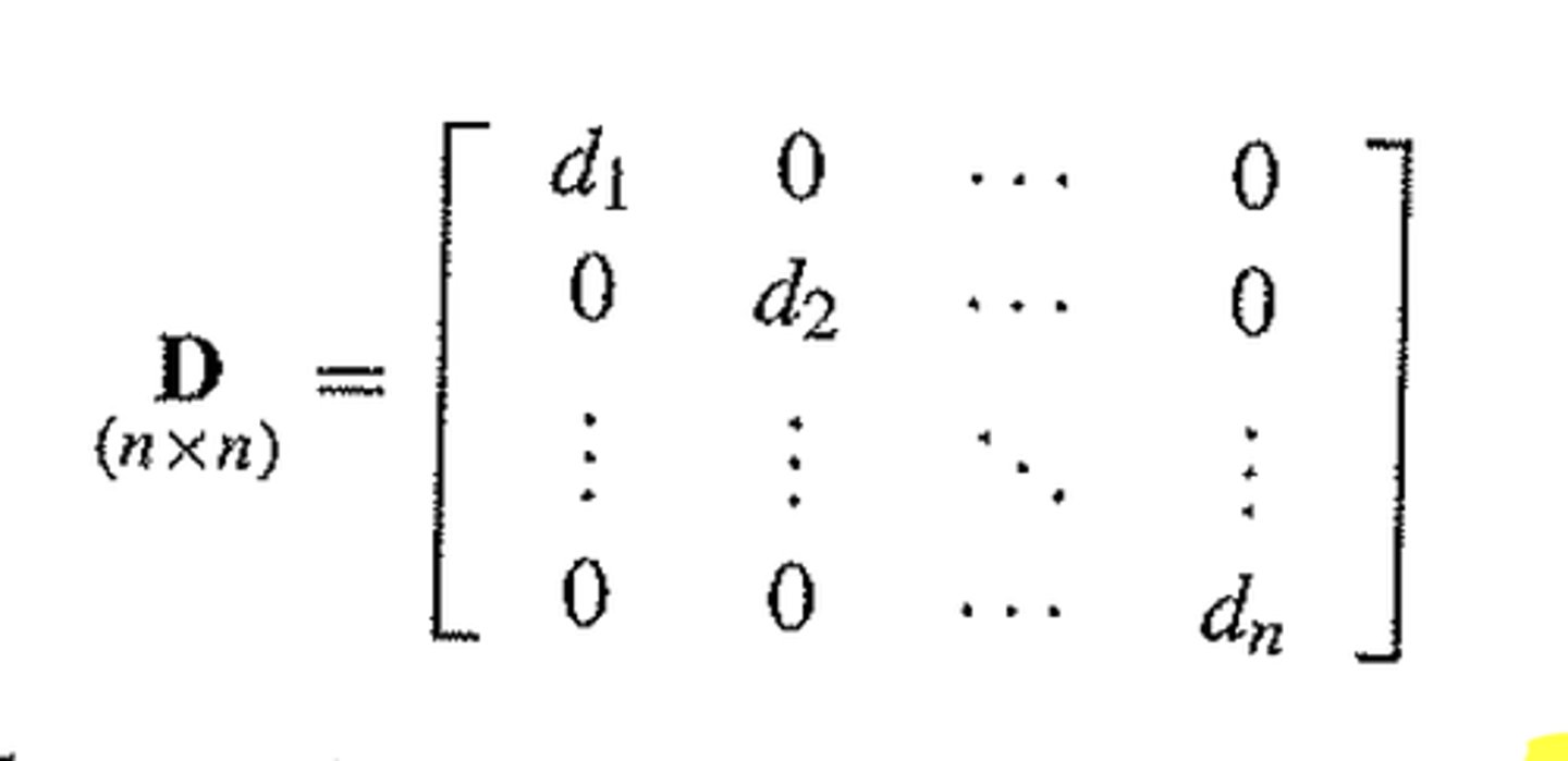
Diagonal matrix:

how to diagonalize M

eigenvalues of a diagonalized matrix

relation to quadric forms

4 useful properties relating Λ and M

X⁻¹MX = Λ where X is the matrix of eigenvectors in the columns ( n × n matrix is diagonalizable iff it has n linearly-independent eigenvectors.)

Diagonalization doesn't change original eigenvalues. and it has them across its diagonal.

Diagonalizing a matrix transforms it into a basis of its eigenvectors (principal axes), which helps quadric form recognition and graphing.

- Powers: Mⁿ=XDⁿX⁻¹

- det(M) = det(Λ) = product of eigenvalues

- tr(M) = dum of eigenvalues

- tr(Mⁿ) = tr(Λⁿ)

Properties of the Eigenvalues and Eigenvectors of an Hermitian Matrix

- The eigenvalues of an Hermitian matrix are real.

- The eigenvectors of an Hermitian matrix with distinct eigenvalues are orthogonal.

- An Hermitian matrix has n orthonormal eigenvectors

to show the first two:

Hx = λx , Hy = µy for two eigenvecs+vals.

y †H = µ ∗ y †

=> y †Hx = λy † x = µ ∗ y † x

=> y †Hx = λy † x = µ ∗ y † x

=> (λ − µ ∗ )y † x = 0

Property of the Eigenvalues and Eigenvectors of

anti Hermitian Matrices

unitary matrices

imaginary

of unit modulus

Normal matrix eigenvector properties

the eigenvectors of normal matrices corresponding to distinct eigenvalues are orthogonal. and a repeated eigenvalue will have an eigenvector for each repeat. its eigenvectors form an orthonormal basis.

what matrices are diagonalizable?

how to diagonalize a matrix?

There are n linearly independent eigenvectors. satisfied automatically for normal (including anti/Hermitian, Unitary, Orthogonal).

use: X †HX = Λ

note: all normal matrices unitarily diagonalizable - X is unitary - all columns (the eigenvectors) are orthonormal.

the eigenvalues of a metric are...

the eigenvectors of a metric are...

strictly positive

the new basis vectors of the diagonalized metric

quadric form:

expression in terms of x

expression in terms of x' (principle basis)

what does quadric form = constant tell us?

, F(x) = x^T S x for real symmetric S and real x

F(x) = x′T Λ x′ = ∑=λₙxₙ² where Λ is the diagonalized S (all cross terms vanish. eg 2x²+3y²+z² = C is an ellipsoid).

we get an equation like in the photo and this can be:

Ellipsoid, Hyperboloids (sand-clock, attached or detached), Paraboloids, Elliptical conical surfaces, planes, cylinders.

the Rayleigh quotient: definition and relation to eigenvalues.

λ(x) = (x^T S x)/(x^T x)

inverse of the distance from a point on a form to the origin, normalized to remove depndence of the constant to which the form was equal.

It is proven that for an hermitian matrix, the values of λ(x) = x †Hx/x†x at its stationary point are the eigenvalues.

Cauchy's principle of convergence

sufficient condition for the sequence sₙ to converge:

for any positive number ε, | s_(n+m) − s_n | < ε for all positive integers m, for sufficiently large n.

Bounded sequences definition

he sequence sn is bounded as n → ∞ if there exists a positive number K such that |sₙ| < K for sufficiently large n

Convergent series

as n → ∞, sₙ tends to a finite limit s. sₙ here is the partial sum sₙ = Σu_r from r₀ to n.

necessary condition for convergence

u_r → 0 as r → ∞

not a sufficient condition for convergence!

Absolute and conditional convergence definitions

absolute:

Σ |u_r| from 1 to ∞ converges.

this implies Σ u_r from 1 to ∞ converges.

conditional: Σ |u_r| diverges and Σ u_r converges.

example: harmonic vs oscillating harmonics

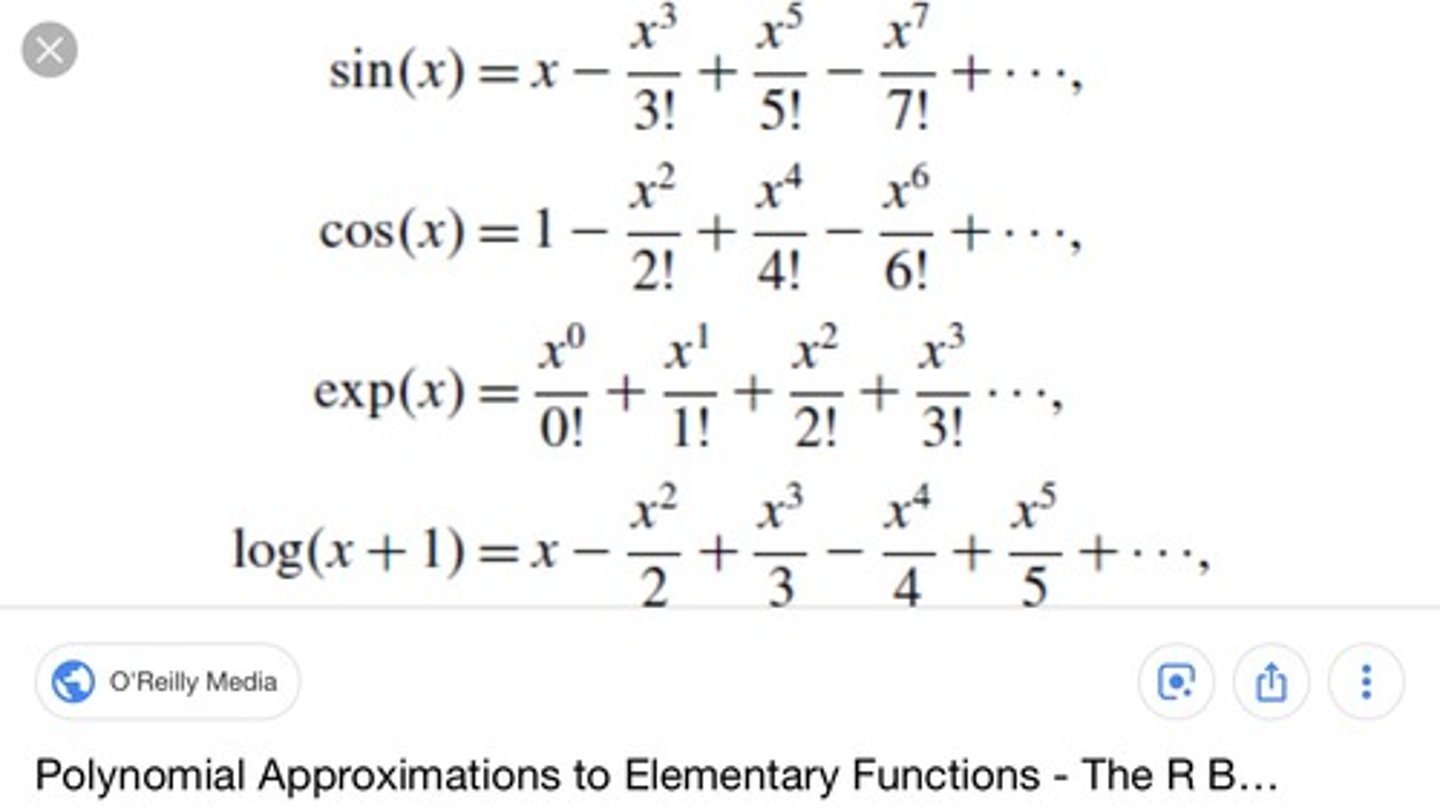
log(1+x), sin(x), cos(x), exp(x) taylor expansions

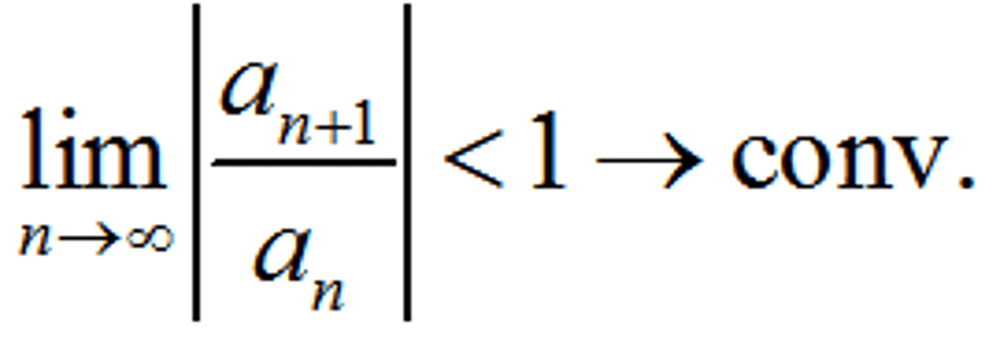
D'Alembert's ratio test

if ϱ = lim u_(r+1) / u_r as r → ∞

Σ u_r converges if ϱ < 1 and diverges for ϱ>1

Cauchy's test

lim u_r ^(1/r) = ϱ as r→∞

Σ u_r converges if ϱ < 1 and diverges for ϱ>1

The O notation

f(z)/g(z) is bounded as z→z0, f(z) = O(g(z)) as z→z0

f(z)/g(z)→0 as z→z0, f(z) = o(g(z)) as z→z0

g(z)/f(z)→1 as z→z0, f(z) ∼ g(z) as z→z0

The Cauchy-Riemann equations (complex derivatives) and concequences

for f(z) = u(x, y) + iv(x, y) , necessary conditions for convergence are -

∂u/∂x = ∂v/∂y , ∂v/∂x = − ∂u/∂y

consequences:

- If we know the real/imaginary part of an analytic function we can find its imaginary/real part up to an additive constant by integrating the Cauchy-Riemann equations.

- If a function of a complex variable is analytic in a region R it is differentiable any number of times in R.

Analytic function

Entire function

examples

Analytic: have a complex derivative at every point z in a region R of the complex plane → analytic in R

entire: analytic in the whole complex plane

examples (entire): any combination of exponentials, polynomials, trig functions. Basically all functions that can be composed of power series, which are all "nice" functions (for example, excluding f(z) = z* )

definitions:

zeros

Poles

connection between zeros and poles

essential singularities

zeros: points where f(z0) = 0 . has order N if all derivatives up to the N-1 give 0: f(z0) = f ′ (z0) = f ′′(z0) =...= f (ⁿ⁻¹)(z0) = 0 . simple zero means N=1.

poles: f(z) has a pole of order n if f(z) = (z − z0)⁻ⁿ g(z) . simple pole means N=1.

If f(z) has a zero of order N at z = z0, then 1/f(z) has a pole of order N there, and vice versa.

essential singularities: if a power series of a function around z0 requires infinite negative powers, z0 is an essential singulaity (unlike removable, which can be removed by multiplying the function by (z-z0)ⁿ.

Radius of convergence:

mathematical definition

physical meaning

how to find

Σ(z − z0)^r converges for |z − z0| < R and diverges for |z − z0| > R

it is equal to the distance of the nearest singular point of the function f(z) from z0.

to find, use D'Alembert's ratio test (if the limit exists)

lim | a_(r+1) / a_r | = 1/R as r→∞

or cauchy's test:

lim | u_r |^(1/r) = 1/R as r→∞

second solution to an ODE using the wronskian and y1

expression for the wronskian

y2 = y1 ∫W(η)/[y1(η)]² dη upper limit: x

W = k exp(-∫p(ζ) dζ ) where p is the coefficient of y' (when the coefficient of y'' is 1).

ordinary, regular singular and irregular singular points of a complex ODE

for a differential equation y ′′(z) + p(z)y ′ (z) + q(z)y(z) = 0 :

ordinary point: if p(z) and q(z) are both analytic at z = z0, then z = z0 is called an of the ODE.

regular singular points: (z − z0)p(z) and (z − z0) 2 q(z) are both analytic at z = z0.

irregular singular points: else.

solving a complex homogenous ODE as a power series around an ORDINARY point

1. assume y = Σaₙzⁿ from 0 to ∞ (origin shift if needed). find y' and y''.

2. if p and q are rational functions (i.e. ratios of polynomials) it is a much better idea to multiply the equation through by a suitable factor to clear denominators.

3. substitute y, y', y'' into the equation.

4. change the sums by substituting r = n-1 or n-2 , to obtain one big sum.

5. since each power coefficient should be zero, obtain a recurrence relation.

6. if needed, find a nicer relation (eg odd and even decoupling) in terms of a0 and a1, and substitute back into y = Σaₙzⁿ.

solving a complex homogenous ODE as a power series around an REGULAR SINGULAR point

1. assume y = Σaₙz^(n+σ) from n=0 to ∞ (origin shift if needed).

2. find s = zp(z) and t = z²q(z) in terms of polynomials or infinite sums.

3. find σ₁ , σ₂ using σ(σ-1)+σs₀+t₀ = 0

4. for each σ, use Σ[ (σ + n)(σ + n − 1) + (σ + n)s(z) + t(z) ]aₙzⁿ =0 to obtain recurrence relation for aₙ.

5. for σ₁ ≠ σ₂ and σ₁ - σ₂ ≠ N , y₁ = z^σ₁ Σaₙzⁿ and y₂ = z^σ₂ Σaₙzⁿ. This also works for σ₁ - σ₂ is an odd integer specificaly for bessel.

6. for σ₁ ≠ σ₂ and σ₁ - σ₂ is an even integer, y₁ = z^σ₁ Σaₙzⁿ for the larger σ , and y₂ = z^σ₂ Σaₙzⁿ + Ky₁ln(z) . This also works for a repeated root.

Variation of Parameters: when is it useful, steps.

Solves any nonhomogeneous ODE (sometimes can't obtain closed form). For y ′′(z) + p(z)y′(z) + q(z)y(z) = f(x):

1. solve the homogenous case with f(x) = 0, and denote the result y_c(x) = c₁y₁(x)+c₂y₂(x). Hence y_p(x) = u₁(x)y₁(x)+u₂(x)y₂(x)

2. compute the wronskian W = y₁y₂′​−y₁′​y₂

3. compute u₁ and u₂ using:

u₁(x) = -∫​y₂(x)f(x)/W(x) dx

u₂(x) = ∫​y₁(x)f(x)/W(x) dx

4. plug u₁(x) , u₂(x) into y_p(x). The final solution to the equation is y_c(x) +y_p(x).