Open Economy

What is new with the open economy?

There are now two stabilisation channels in an open economy. Firstly, following a shock where π > πT the CB will, like before, raise interest rates to create a negative output gap and reduce inflation.

However, when a CB decides to change its interest rate then an arbitrage opportunity arises where traders can profit from the interest rate differential.

If, for example, the FX market expects the BoE to increase the UK interest rate then the return on UK bonds will be higher than on US bonds. This will lead investors to buy UK pounds and sell US dollars, leading to the UK currency appreciating, until the arbitrage opportunity disappears. This currency appreciation means that net-exports and AD will fall, reducing output and helping to lower inflation.

Thus, the FX market now has a role to play, alongside the CB, in stabilising the economy after a shock and the CB has to raise the interest rate i by less than in the closed economy model.

So what is the key determinant of exchange rate fluctuations?

The key determinant of exchange rate fluctuations is the buying and selling of currencies in the FX market to trade government bonds of different countries.

How has the IS, PC and MR changed in the open economy?

The IS curve now includes imports and exports and so is steeper (has a lower multiplier) because some of the effects of an interest rate change will leak abroad. In a closed economy, a reduction on interest rates will lead people to spend more and this expenditure will remain within the native economy. However, in an open economy some of this increased spending will be on imports.

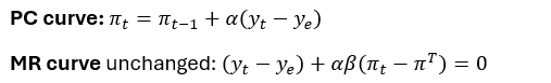
PC and MR will be kept fundamentally the same.

What is the nominal exchange rate?

The Nominal exchange rate E = no. units of home currency / one unit of foreign currency. aka how many pounds per one dollar.

An increase in E corresponds to a depreciation of home currency.

e = ln(E)

What is the real exchange rate?

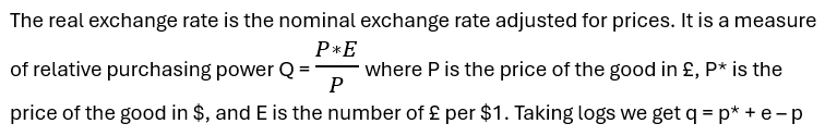
Explain purchasing power parity:

Arbitrage in international markets should mean that traded goods have the same price irrespective of location. This is the Law of One Price (LOP) where P = P*E ←→ Q = 1. If this applied to all goods, and baskets of goods were equal across countries, this would imply absolute purchasing power parity.

However, this absolute PPP never actually applies. Instead we could have relative PPP where Q is not equal to one but remains constant. For example, prices in one country might always be 20% higher because of e.g. tariffs, transport costs, but Q = 1.2 will always stay the same.

In practice, there is little evidence for either absolute or relative PPP as q rarely stays constant and has shown to be capable of changing a great deal.

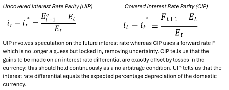
What is the UIP and CIP equations, and explain the difference:

What are the first two assumptions under which the UIP holds?

1.      We assume perfect international capital mobility

In reality, transaction costs, capital controls, and institutional regulations prevent money from flowing as frictionlessly as the theory suggests.

That being said, the UK, specifically the City of London, is one of the most open financial centres in the world with no major capital controls.

2.       We assume a small home country which cannot affect world interest rates

This fails for economies like the US, China, or the EU, where domestic policy shifts significantly move global interest rates and credit conditions.

What are the second two assumptions under which the UIP holds?

3. We assume that households can hold two assets: bonds (both home and foreign) and money.

This of course majorly oversimplifies modern portfolios, which include real estate, equities, and commodities, all of which react differently to inflation and interest rates than cash or bonds.

4. We assume perfect substitutability between home and foreign bonds. This means that the riskiness of foreign and home bonds is identical, so the only relevant difference between them is the expected return.  This depends on two factors: any expected difference in interest rates over a specific time horizon, and an expectation about the likely development of the exchange rate over that same time horizon.

In reality, sovereign and liquidity risk is a major and very real consideration. Investors would rarely view a 10-year bond from a volatile emerging market as identical in risk to a US Treasury note.

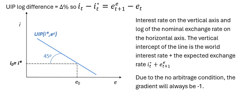
How can we show the UIP graphically:

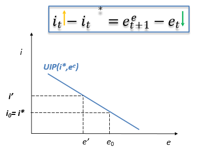
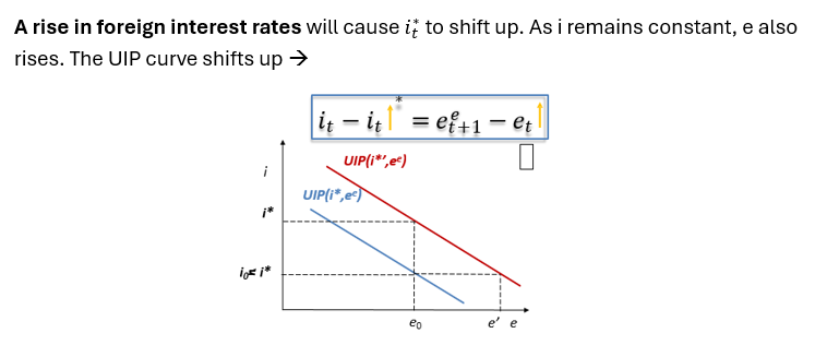
What happens on the UIP graph after a rise in home interest rates?

A rise in home interest rates will not shift the intercept but will only cause a movement along the existing UIP line.

What happens on the UIP graph after a rise in world interest rates?

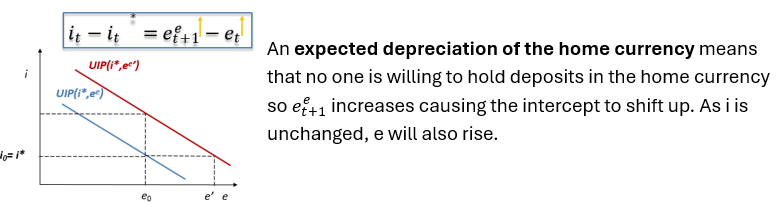
What happens on the UIP graph after an expected depreciation of the home currency?

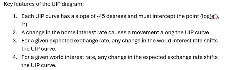
Summarise the four key features of the UIP diagram:

BoE suddenly raise interest rates by 2.5%. Show the effects of this on interest rates and exchange rates over time

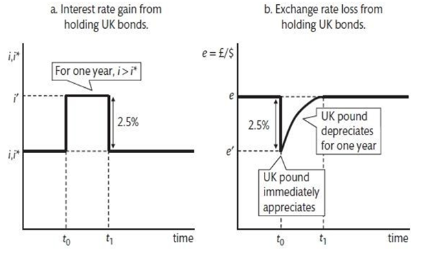
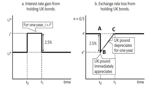
Explain what happens when the BoE suddenly raise interest rates by 2.5%. 

BoE suddenly raise interest rates by 2.5%. This makes UK bonds more attractive so investors will sell USD and buy GBP in order to take advantage of this expected return. This leads the US dollar to depreciate and the UK pound to appreciate immediately by 2.5%.

Studies find that any arbitrage opportunities that arise as a result of interest rate differentials (or expected differentials) are exhausted within a matter of seconds.

Explain what happens at point B:

The UIP condition tells us that the interest gain from holding UK bonds over US bonds = the loss from the expected UK currency depreciation against the US’.

As soon as the interest differential is no-longer greater than the currency loss, forex traders have no incentive to buy UK bonds. Point B is this point where the two balance.

Explain what happens between B and C, and where the gradient comes from?

As we approach the time when the interest rate differential will disappear, the size of the interest gain from a UK bond shrinks and hence the matching expected depreciation of the pound must be smaller. The exchange rate must therefore be closer to its expected level of e. Assuming that everything after the surprise change in interest rates is known with certainty, the transition path from B to C will be a smooth one. The gradient of CB is given by the UIP.

What would happen if there was no interest rate differential at any time but the long run exchange rate changes?

The exchange rate on the RHS graph would jump to its new long run value as soon as the new long-run value is expected (no triangle).

What happens if there is a new long run exchange rate and an interest rate differential (essentially moving point C up or down).

Imagine there is a new long run exchange rate and an interest rate differential (essentially moving point C up or down).

The gradient of the transition path is determined by the interest rate differential via UIP, as before, and must meet the new long run value smoothly. Thus, the important change is the size of the initial jump from A to B. If the long-run target (C) moves up or down, the starting jump (B) must move by the same amount to maintain the correct gradient.

What happens in the original case if the interest differential is anticipated before t0 when it actually happens at point A?

The “vertical jumps in response to new information” rule tells us that the exchange rate will jump down immediately to the level of B and then stay flat until B is reached (there is no interest differential at the time so no gradient). It will then follow the BC path as before.

Why does this representation not match up with reality?

In practice, exchange rates will react almost continuously to changes in the expectations of future interest rate differentials and changes in expected long run exchange rates. New information will affect exchange rates in very volatile, immediate ways. A real-world graph would show constant vertical jumps and shifting gradients as traders constantly recalculate Point B and Point C based on new information.

Describe the difference between the short run and the medium run:

In the short run, prices (and wages) are fixed so the CB uses r to stabilise output.

In the medium run, prices of factors of production are allowed to adjust to demand and supply in their respective markets. For example, wages adjust to the demand and supply of labour. Real output and income are determined by the economy’s productive capacity not by monetary policy.

What are three further assumptions for our open economy model?

1. Small open economy where r is ultimately fixed by the world interest rate r*

This ignores risk premiums. Even if the world rate is 2%, a country with political instability might have to offer 5% just to get people to hold its bonds. It also assumes the country is too small to nudge the global rate.

2. Exchange rate regime, either:

   -            Fixed: e is pegged to a foreign currency giving no autonomy of monetary policy

   -            Floating: e is determined by UIP

3. The home market’s inflation target is equal to a constant world inflation Otherwise e would not be stable as implies a constantly appreciating nominal exchange rate.

Countries often deliberately choose different inflation targets based on their specific developmental needs, accepting that their currency will gradually drift in value over decades.

What is the new IS curve?

Explain the aspects of this new IS curve:

A represents autonomous demand: the baseline spending from households, firms, and the government that doesn’t depend on interest rates or the exchange rate.

Interest rate effect. If interest rates were high in the previous period, investment and consumption drop today.

Exchange rate effect. q represents the real exchange rate. If q goes up, it means the currency has depreciated (become weaker). Domestic goods become cheaper for foreigners to buy (exports increase), and foreign goods become more expensive for you (imports decrease). Hence, net exports rise, which boosts total output.

What is the PC and MR curves?

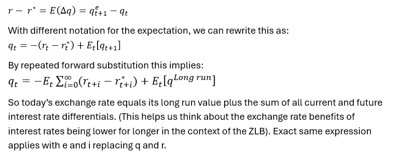
Write the nominal UIP condition, and then the real UIP condition:

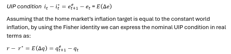
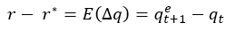
Derive this equation further:

Show and explain the AD side of the economy when CB cuts interest rates:

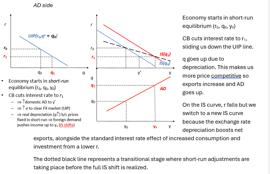
What does each AD curve represent? What moves us along or shifts the AD curve?

Each AD curve represents a short-run equilibrium

-            Monetary policy moves us along the AD. When the Central Bank cuts r, the UIP condition forces q to rise, moving us down the AD curve to a higher level of output.

-            Fiscal policy (Government spending or taxes) or other demand shocks (like a sudden rise in consumer confidence) change the autonomous demand A in the IS equation, and thus shifts the AD. Fiscal policy changes the level of output for any given interest rate.

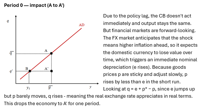
Suppose the economy starts at the inflation target. What happens immediately after a cost-push shock?

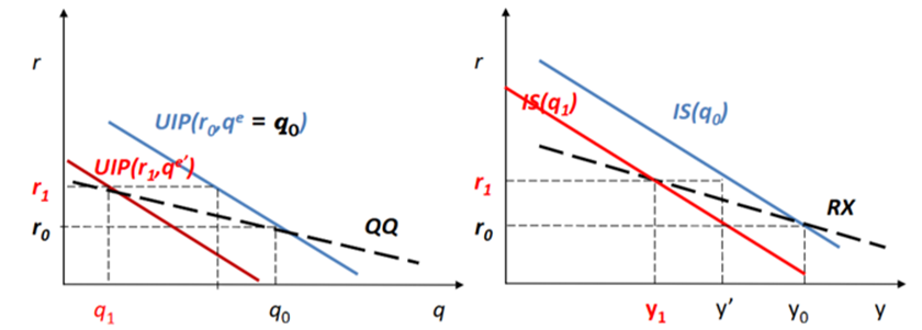
Draw the subsequent UIP and IS adjustments:

What happens in period 1?

The CB now raises interest rates to create a negative output gap and push inflation back toward target.

But here is where the open economy complicates the simple story: the IS curve includes the exchange rate term (+bq), meaning the real appreciation at A' has already dampened demand by squeezing net exports. Hence, the CB needs to raise r by less than it would in a closed economy to achieve the same disinflationary effect. This is the RX curve logic - the CB is not just moving along a fixed IS curve, but operating on a curve that shifts with exchange rate movements.

Simultaneously, because the FX market knows the CB will fight the shock, it anticipates a sustained period of higher rates followed by a gradual cut. This expectation of future appreciation shifts the UIP curve to the left immediately.

The CB sets r1 - lower than the closed economy equivalent - and this intersects the new IS position at point B.

What happens in the subsequent periods?

As the CB gradually cuts rates in subsequent periods, the FX market revises its expectations of appreciation downward - the UIP curve shifts back to the right each period. r falls, q depreciates back toward its original level, net exports recover, and output rises back to equilibrium as inflation returns to target. This back-and-forth is captured by the QQ line, which maps out all the (r, q) combinations along the adjustment path: r goes up then back down, q goes down then back up, and the UIP intercept mirrors this throughout since the The FX market is aware of this dynamic and their expectations mirror this.