STATS One-way within-subjects (repeated measures) ANOVA

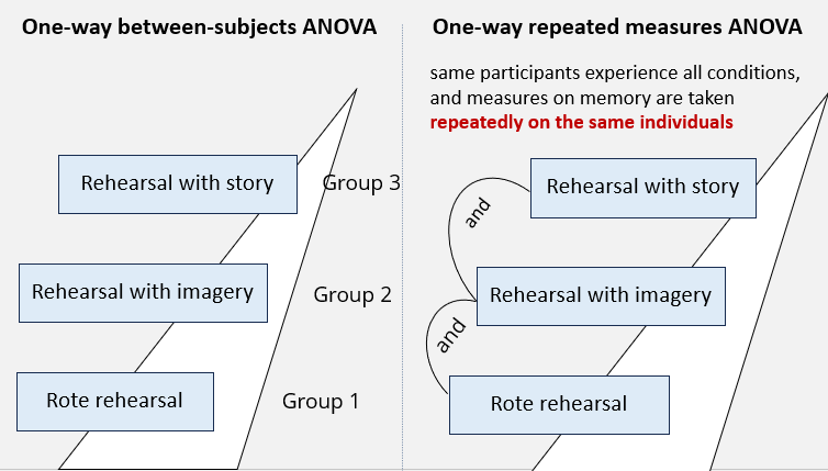
Difference between between-subjects ANOVA and within-subjects ANOVA

Between-subjects design

• Each participant appears under only one level/condition

• One IV

Within-subjects design

• Same participants appear in ALL conditions

• One IV

Evaluation of Between-subjects (independent groups) ANOVA

PROS:

• Simplicity

CONS:

• Large variability from person to person: there could be one participant that is really eager than the other

• Requires large sample sizes for power

Evaluation of One-way within-subjects (repeated measures) ANOVA

PROS:

• More economical - fewer cases

• Controls for individual differences

• Providing relatively accurate estimates - accurate detecting the effect of the conditions or treatments being tested

CONS:

• Carryover effects - exposure to treatment at one time influences responses to another

• Practice effect

• Fatigue effect

3 Assumptions for one-way within-subjects (repeated measures ANOVA)

1. Levels of measurement - DV is continuous

2. Normality of residuals - Residuals are normally distributed close to the reference line on a QQ plot

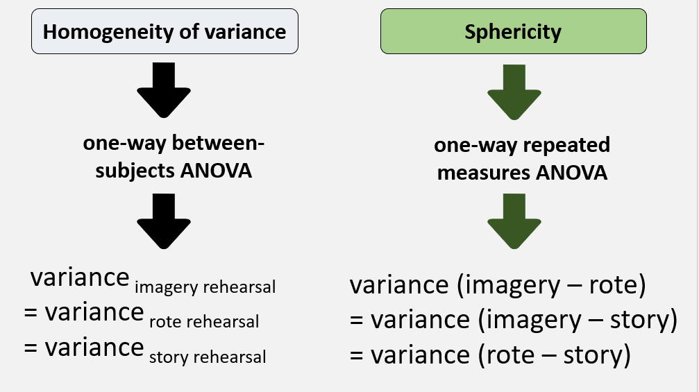
3. Assumption of sphericity

Sphericity

Variance of differences between any two conditions must be the same as the variance of the differences between any other two conditions

• Variance of the differences between Rote rehearsal and Story rehearsal  

=  

• Variance of the differences between Rote rehearsal and Imagery rehearsal 

= 

• Variance of the differences between Story rehearsal and Imagery rehearsal 

Instead of looking at the 3 groups seperately (homogeneity of variance), sphericity looks at the variances with each pair making sure its equal

Uses Mauchly’s test

Mauchly’s test for Sphericity and its violations

W statistic = .xx, p = .xx

If p < .05, the assumption of sphericity is violated

If p > .05, the assumption of sphericity is satisfied

Without sphericity, we are in danger of making Type II errors → the test therefore loses statistical power → test is less sensitive to detecting true differences

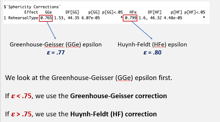
Sphericity correction if the assumption is violated

Greenhouse-Geisser (GG) correction or Huynh-Felt correction (HF)

Epsilon (𝜺) : sphericity estimate → under GGe or HFe in R

• Measures how far the data is from the ideal sphericity

• Ranges between 0 and 1 (1 = no violation of sphericity)

Look at the Greenhouse-Geisser (GGe) epsilon first

• If 𝜺 < .75, we use the Greenhouse-Geisser correction

• If 𝜺 > .75, we use the Huynh-Feldt (HF) correction

Therefore, if sphericity is violated, only report the scores AFTER the sphericity correction

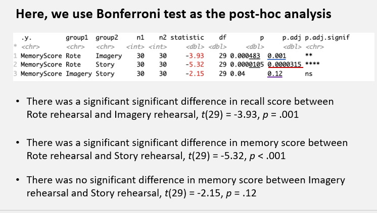
What is the post hoc test for one-way within-subjects ANOVA?

Bonferroni method

t(df) = statisticx.xx, p = p.adj.xxx

What do you do after the post-hoc analysis for one-way within-subjects ANOVA?

You already have the generalised effect size for the overall ANOVA (η_G² generalised eta squared), you also need to calculate the effect size (Cohen’s d) for each of the pairwise comparison

Write-up

We conducted a one-way repeated measures ANOVA to test the effect of rehearsal types on memory performance.

Mauchly’s test of sphericity revealed a violation of sphericity (p = .006). A one-way repeated measures ANOVA with a Huynh-Fedlt correction suggested a significant effect of rehearsal types on memory performance, F(1.6, 46.32) = 14.57, p < .001, , η_G² = .14.

Bonferroni-adjusted pairwise comparisons showed that students using the rote rehearsal strategy had significantly lower memory performance compared to those using the imagery rehearsal strategy (t(29) = -3.93, p = .001, d = -.72) and those using the story rehearsal strategy (t(29) = -5.32, p < .001, d = -.97). However, there was no significant difference between the imagery and story rehearsal strategies (t(29) = -2.15, p = .12, d = -.39).

When do you omit the 0 before a decimal point in a write up?

If the number can exceed 1, you keep the 0 (F-value, pairwise comparisons)

If the number cannot exceed 1, omit the 0 (correlations, epsilons, effect sizes, p values)

Note: for zeros after decimal points, always include trailing zeros even after 1 significant figure (to ensure that it is 2 significant figures)

How do you know the direction of a pairwise comparison?

If the cohen’s d is positive (positive effsize), then group 1 has a higher mean than group 2

If the cohen’s d is negative (negative effsize), then group 1 has a lower mean than group 2

If sphericity is violated, which results do you include/exclude?

Use the corrections degrees of freedom and p-value

Keep the original F-value and generalised effect size